Italian elections (1)

You’d think that the last week before the holidays would be very quiet and not much would be going on. Well, if you did, you’d be wrong, I guess, as the last few days have been quite busy (for many reasons).

Anyway, I managed to track down some better data on a set of recent polls for the upcoming Italian elections. Most of the public sites I found had a basic table with the proportions representing the voting intentions for a set of units sampled in a given poll. This means that the actual sample size (or any other information about the poll) is in general not present, making it impossible to appreciate any form of uncertainty associated with the estimations.

I think I may be able to get good quality information from YouTrend.it, who collect this kind of information too (although it is not directly present in the data that are publicly available). This would be good; and we may be able to update the estimations in some clever way, as more polls are conducted closer to the actual date of the elections.

But in the meantime I’ve compiled a list of the polls conducted after October and, for nearly all of them, I was able to link the sample size. This was by no means systematic, as I was trying to get what was available and usable; on the plus side, however, I think that I actually got most of the reasonably sized ones. The resulting dataset consists of $N=45$ polls, collecting voting intentions for $J=11$ parties, which will all take part in the “event”.

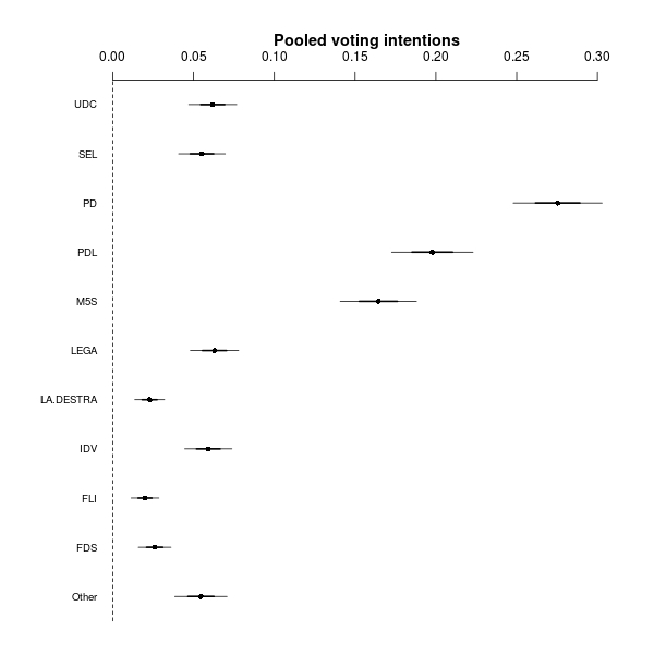
I’ve hastily run a relatively simple multinomial regression model. For each poll, I modelled the observed vector of voting intentions ${\mathbf{y}}_i=(y_{i1},\dots ,y_{iJ})$ as $${\mathbf{y}}_i\sim \text{Multinomial}({\mathit{\pi }}_i,n_i)$$ where ${\mathit{\pi }}_i=({\pi }_{i1},\dots ,{\pi }_{iJ})$ is the vector of polls- and party-specific probabilities; each of them is defined as $${\pi }_{ij}=\frac{{\varphi }_{ij}}{\sum _{j=1}^J{\varphi }_{ij}}.$$ The elements ${\varphi }_{ij}$ represent some sort of “un-normalised” probabilities (voting intentions) and for now I have modelled them using a convenient log-linear predictor $$\log ({\varphi }_{ij})={\alpha }_j+{\beta }_{ij}.$$ The parameters ${\alpha }_j$ are the “pooled estimation” of the (un-normalised) voting intentions for party $j$ (where pooling is across the $N$ polls), while the parameters ${\beta }_{ij}$ are poll-party interactions. For now, I gave them vague, independent Normal priors and I re-scaled the ${\alpha }_j$’s to obtain an estimation of the pooled probabilities of votes for each party $${\theta }_j=\frac{\exp ({\alpha }_j)}{\sum _{j=1}^J\exp ({\alpha }_j)}.$$ Although relatively quick and dirty, the model gives some interesting results. Using the coefplot2 package in R, one can summarise them in a graph like the following.

The dots are the means of the posterior distributions, while the light and dark lines represent, respectively, the 50% and 95% interval estimations. Much as I thought before, the interesting thing is that the Democratic Party (PD) seems to have a firm lead, while the two parties fiercely competing for the worst name ever to be bestowed upon a political party, Berlusconi’s PDL (which translates as “Freedom People”) and M5S (“5 Stars Movement”) are also competing fiercely for the same chunk of votes. Also, there’s a myriad of small parties, fighting for 2%-5%.

Of course, the model is far from ideal $-$ for example, I think one could model the parameters ${\alpha }_1,\dots ,{\alpha }_J\sim \text{Normal}(\mathit{\mu },\mathbf{\Sigma })$ to account for potential correlation across the parties. This for example would make it possible to encode the fact that those showing intention to vote for PD are very unlikely to then switch to PDL.