Zero to hero

Recently, I’ve been working on a paper, which I think is coming along nicely. The basic problem is like this: in a health economic evaluation, sometimes data are collected on a sample of individuals. Say, for example, that $n_0$ subjects are given a standard treatment $t=0$ and $n_1$ are treated with a new intervention $t=1$. For each subject, we typically observe a measure of clinical benefit $e_i$, which tells us how “good” the treatments are, and a measure of overall cost $c_i$.

Costs (and for that matters benefits) are almost invariably associated with skewed distributions (and thus suitable models are Gamma and log-Normal) and, generally $(e,c)$ are actually correlated. Moreover, sometimes, for some of the patients, $c_i=0$, ie some people are observed to accrue no costs to the NHS. For these, you can’t really use a Gamma or a log-Normal.

In the paper, I extend the framework of hurdle models commonly used to tackle the issue of individual patients with observed zero costs, to include a full cost-effectiveness model, accounting for correlation between costs and a suitable measure of clinical effectiveness (eg QALYs). Basically, I do this using a structure consisting of:

1. a selection model for the chance of observing a zero cost, typically as a function of some individual covariates (eg age and sex);
2. a marginal model for the costs, inducing a mixture (of subjects with 0 cost and subjects with positive costs), depending on the selection model;
3. a conditional model for the benefits, depending on the costs (so that correlation between $e,c$ is guaranteed).

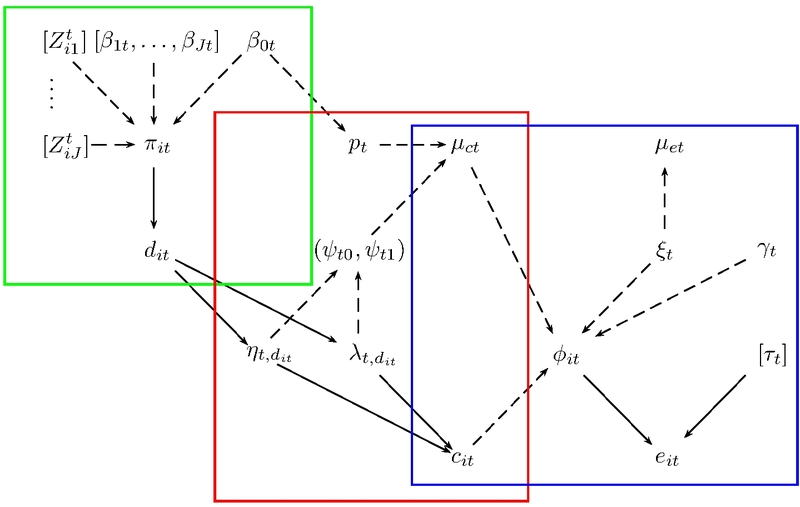
In graphical terms, something like this.

The green part is the selection model, estimating the overall average probability of a zero cost, which is used to weigh the components of the mixture model (in red). The observed costs have a distribution which is characterised by two parameters ($\eta$ and $\lambda$). These are modelled so that they induce a mean and variance of 0 for those subjects for whom the observed value is 0, and a proper (Gamma or log-Normal) distribution for the others. Finally, the blue part is the model for the benefits, which is defined as a (possibly generalised) linear regression, depending on the costs. The parameters $({\mu }_c,{\mu }_e)$ are then used to do the cost-effectiveness analysis, eg using BCEA.

I’ve prepared a R package that would use this framework to do this analysis. I’m allowing for some possible distributions for both $c$ (Gamma and log-Normal) and $e$ (Beta, Bernoulli, Gamma and Normal). The package (which I’m provisionally calling BCES0, for Bayesian Cost-Effectiveness for Structural 0s) lets you select the distributional assumptions and then builds a model code and runs it in JAGS. The user doesn’t even know how to code JAGS models (provided they’re happy with the relative general model that will be produced automatically). But I’m making R save the model file, so that you can actually see it and modify it as needed.

I’ll post more once I’ve debugged the package and prepared a couple of nice examples (I’ll put a working paper in here soon). I’ll also give a talk on this at the LSHTM in the autumn $-$ more on this later!