The greedy baker with a full barrel and a drunken wife

Earlier this week, I gave a talk at one of the UCL Priment seminars. The session was organised around two presentations aimed at discussing the definition and differences between “confidence” and “credible” intervals \(-\) I think more generally, the point was perhaps to explore a little more the two approaches to statistical inference. Priment is a clinical trial unit and the statisticians and clinicians involved there mostly (if not almost always) use frequentist methods, but I think there was some genuine interest in the application of Bayesian inference. I enjoyed very much the event.

For my talk, I prepared a few slides to briefly show what I think are the main differences in the two approaches, mostly in terms of the fact that while in a Bayesian context inference is performed with a “bottom-up” approach to quantify and evaluate \[\Pr(\mbox{parameters / hypotheses} \mid \mbox{observed data})\]a frequentist setting operates in the opposite direction using a “top-down” approach to quantify and evaluate \[\Pr(\mbox{observed data / even more extreme data} \mid \mbox{hypothesised parameters}).\] I think that went down well and at the end we got into a lively discussion. In particular, the other speaker (who was championing confidence intervals), suggested that when the two approaches produce results that are numerically equivalent, then in effect even the confidence interval can be interpreted as to mean something about where the parameter is.

I actually disagree with that. Consider a very simple example, where a new drug is tested and the main outcome is whether patients are free from symptoms within a certain amount of time. You may have data for this in the form of \(y \sim \mbox{Binomial}(\theta,n)\) and say, for the sake of argument that you’ve observed \(y=16\) and \(n=20\). So the 95% confidence interval is obtained (approximately) as \[\frac{y}{n} \pm 2\,\mbox{ese}\!\left(\frac{y}{n}\right),\] where ese\((\cdot)\) indicates the _estimated standard error _for the relevant summary statistics.

The probabilistic interpretation of this confidence interval is \[\Pr\left(a \leq \frac{y}{n} \leq b \mid \theta = \frac{y}{n} \right) = 0.95\] and what it means is that if you’re able to replicate the experiment under the same conditions, say 100 times, then 95 of them the resulting confidence interval would be included between the lower and upper limits \(a\) and \(b\). With the data at hand, this translates numerically to \[\Pr\left(0.6211\leq \frac{y}{n} \leq 0.9788 \mid \theta=0.80\right) = 0.95\] and the temptation for the greedy frequentist is to interpret this as a statement about the likely location of the parameter.

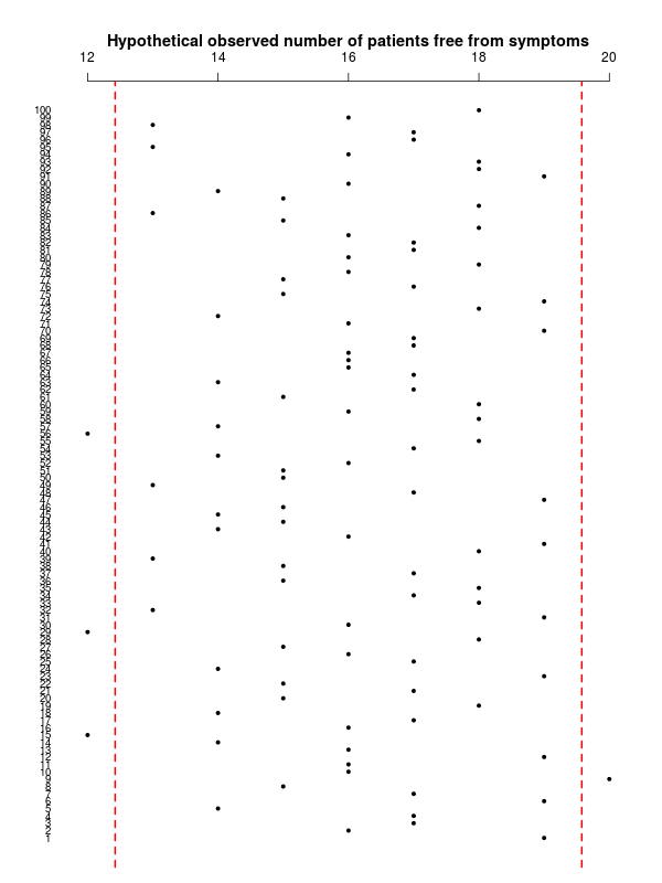
The trouble with this is that by definition, a confidence interval is a probabilistic statement about sampling variability in the data \(-\) not about _uncertainty in the parameters _as shown in the graph below.

(in this case, in fact 4 out of 100 hypothetical sample means fall outside the confidence interval limits, but this is just random variation).

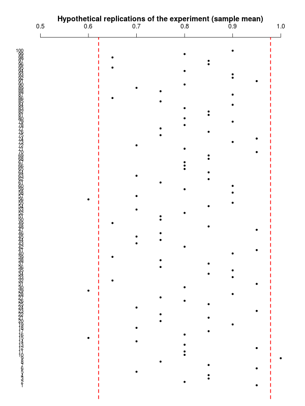
The “alternative” interpretation, rescales the graph above by using the sample mean to produce the one below.

While this is perfectly valid from a mathematical point of view, however, this interpretation kind of muddies the water, I think, because it kind of confuses the point that this is about sampling variability in the data. And the data you would get to see in replications of the current experiment would be about the observed number of patients free from symptoms, \(y^{new} \sim \mbox{Binomial}(\theta=0.8,n=20)\).

Thus, it is a bit confusing, I think, to say that a Bayesian analysis could yield the same _numerical _results as the confidence interval \(-\) perhaps a more appropriate interpretation would be that this is a probabilistic statement in the form \[ \Pr\left(na \leq y \leq nb \mid \theta=\frac{y}{n}\right) = 0.95, \] which in the present case translates to \[ \Pr\left(12.43 \leq y \leq 19.58 \mid \theta=0.8\right) = 0.95, \] which suggest we should expect to see a number of patients free from symptoms between 12 and 20 in replications of the current experiment (which is of course in line with the first graph shown above, on the scale of the observable data).

The Bayesian counterpart to this analysis may assume a very vague prior on \(\theta\), for example \(\theta \sim \mbox{Beta}(\alpha=0.1,\beta=0.1)\). This would suggest we’re encoding our knowledge about the true probability of being symptoms-free in terms of a thought experiment where \(\alpha+\beta=0.2\) patients were observed and only \(\alpha=0.1\) were symptoms free (ie a prior estimate of 0.5 with very large variance).

Combining this with the data actually observed \(y=16, n=20\), produces a posterior distribution \(\theta\mid y \sim \mbox{Beta}(\alpha^*=\alpha+y, \beta^*=n+\beta-y)\), or in this case \(\theta \mid y \sim \mbox{Beta}(16.01,4.1)\), as depicted below.

A 95% “credible” interval can be computed analytically and as it turns out it is \([0.6015; 0.9372]\), so indeed very close to the numerical limits obtained above when rescaling to the sample mean \(y/n\) \(-\) incidentally: 1. It is possible to include even less information in the prior and so get even closer to the frequentist analysis; 2. However, even in the presence of large data that probably will overwhelm the prior anyway, is it necessary to be soooo vague? Can’t we do a bit better and introduce whatever prior knowledge we have (which probably will separate out the two analyses)? 3. I don’t really like (personally) the term “credible” interval. I think it’s actually un-helpful and it would suffice to call this an “interval estimate”, which would highlight the fact that given the full posterior distribution, then all sorts of summaries could be taken.

The Bayesian analysis tells us something about the unobservable population parameter given the data we’ve actually observed. We could predict new instances of the experiment too, by computing \[ p(y^{new}\mid \theta,y) = \int p(y^{new}\mid \theta)p(\theta\mid y) \mbox{d}\theta. \] This means assuming that the new data have the same data generating process as those already observed and that we propagate the revised, current uncertainty in the parameter to the new data collection. In some sense, this is even the “true” objective of a Bayesian analysis, because parameters typically don’t “exist” and they are just a convenient mathematical feature we use to model observable data.

The confidence interval can make probabilistic statements about the likely range of observable data in similar experiments that we may get to see in the future. The Bayesian analysis tells us something about the likely range of the population parameter, given the evidence observed and our prior knowledge, formally included in the analysis.

While I think the construction of the confidence interval has some meaning when interpreted in terms of replications of the experiment (particularly with respect to the actual data!), I believe that the stretch to the interpretation as a probability for the parameter is a unwarranted, hence the reference to the greedy baker who wants to have and eat his cake \(-\) which in Italian would translate as having a full barrel (presumably of wine) and a drunken wife…

So I guess that, in conclusion, if you enjoy a tipsy partner, you should be Bayesian about it…