2  Introduction to R

Howard Thom
University of Bristol, UK

David Phillippo
University of Bristol, UK

2.1 Introduction to the introduction

In this chapter we will give an introduction to the R commands and functionality needed to make the most of this book. We will cover the following topics:

• Rstudio
• Basic operations
• Variables
• Installing and loading packages
• Vectors
• Matrices
• for loops
• Distributions and generating samples
• Saving graphical outputs
• Data types — data frames, arrays, and lists
• Importing and exporting data
• Functions and control flow

Not all of these topics are necessary to follow any individual chapter. All chapters make use of basic operations, variables, and packages but only some use, for example, for loops, data frames, or functions. If you are new to R we would recommend working through this whole chapter carefully. It will give a good grounding in the use of R and give you confidence to tackle any of the subsequent chapters. Even if you do not plan to use certain topics, for example lists or control flow, It is very good to be aware that such functionality exists. A package you use later may rely on lists for its interface, or an algorithm might only be possible if you can use an if statement. The same applies to all the topics in this chapter.

If you wish to learn more about R, there are a wealth of materials available online, including the excellent and freely-available books by Wickham (2019) and Wickham et al. (2023), which are available at https://adv-r.hadley.nz and https://r4ds.hadley.nz, respectively.

We give similar advice to those who are familiar with R, particularly those who are used to R as programme for statistical analysis rather than HTA or modelling. It is best to skim this chapter and read carefully any topics with which you are unfamiliar. R for HTA can be quite different to R for statistics; regression models (see Section 4.6, Chapter 5 and Chapter 6) using the glm() function from the stats package are a fundamental tool for statisticians working with R, but a health economist building Markov models (Chapter 9) might have much less familiarity with them. Conversely, matrices and random sampling are essential for modellers, but a statistician analyzing trial data could get on quite well without them.

A final point to make is that the best way to learn a statistical programming language, or indeed any programming language, is to play and experiment with it. Reading our explanations will only teach you to read R, but experimentation will teach you to use R.

Good luck!

2.1.1 Tidyverse Style Guide

In this chapter we aim to follow the Tidyverse Style Guide for consistency of coding conventions: https://style.tidyverse.org/ — this is mentioned in several other parts of this book (for example Chapter 4, Section 4.6, Chapter 6, Chapter 7 and Chapter 14).

In naming variables and other objects we will use lowercase letters with underscores separating words, for example name_of_variable. The technical term for this convention is snake case.

We include spaces when writing complex expressions to ease readability. This includes spaces after commas, assignments and between mathematical operations.

x <- 3
z <- c(1, 3)
x + z
(x * z) / 2

We also add spaces before and after brackets () and when using if, for, or while control flow operations.

if (TRUE) {
  show(x)
}

Our only departure from the Tidyverse Style Guide is that we choose to include a return() statement at the end of functions. We do this to avoid ambiguity about what the output of a function is, which eases debugging of complex functions.

Tip on coding style

A final stylistic tip when writing scripts is to avoid hard-coding variables. For example, instead of

net_benefit <- qaly * 20000 - cost

it is recommended to instead write

threshold <- 20000
net_benefit <- qaly * threshold - cost

As well as being easier to read and reducing mistakes, this makes it simpler to turn things into functions later.

2.2 Rstudio

R can be run from the (Windows, Mac, or Linux) command line, or from within the included R Graphical User Interface (GUI). However, we recommend using the Rstudio Integrated Development Environment (IDE), developed by the company Posit (RStudio Team, 2020). This provides various “quality of life” aids for programmers, including highlighting of R keywords, automatic indentation, syntax error checks, project functionality for bundling multiple R scripts together, and integrated version control with git (see Chapter 14). Beyond this assistance with the use of base R, Rstudio also has built-in support for markdown (Xie et al., 2018), quarto (Allaire et al., 2024), shiny (see again Chapter 14) and other popular extensions to R. It is not essential to use Rstudio to follow this chapter, or to get the most out of this book, but it will likely make your learning and working much easier.

The overall interface for the Rstudio IDE is illustrated in Figure 2.1.

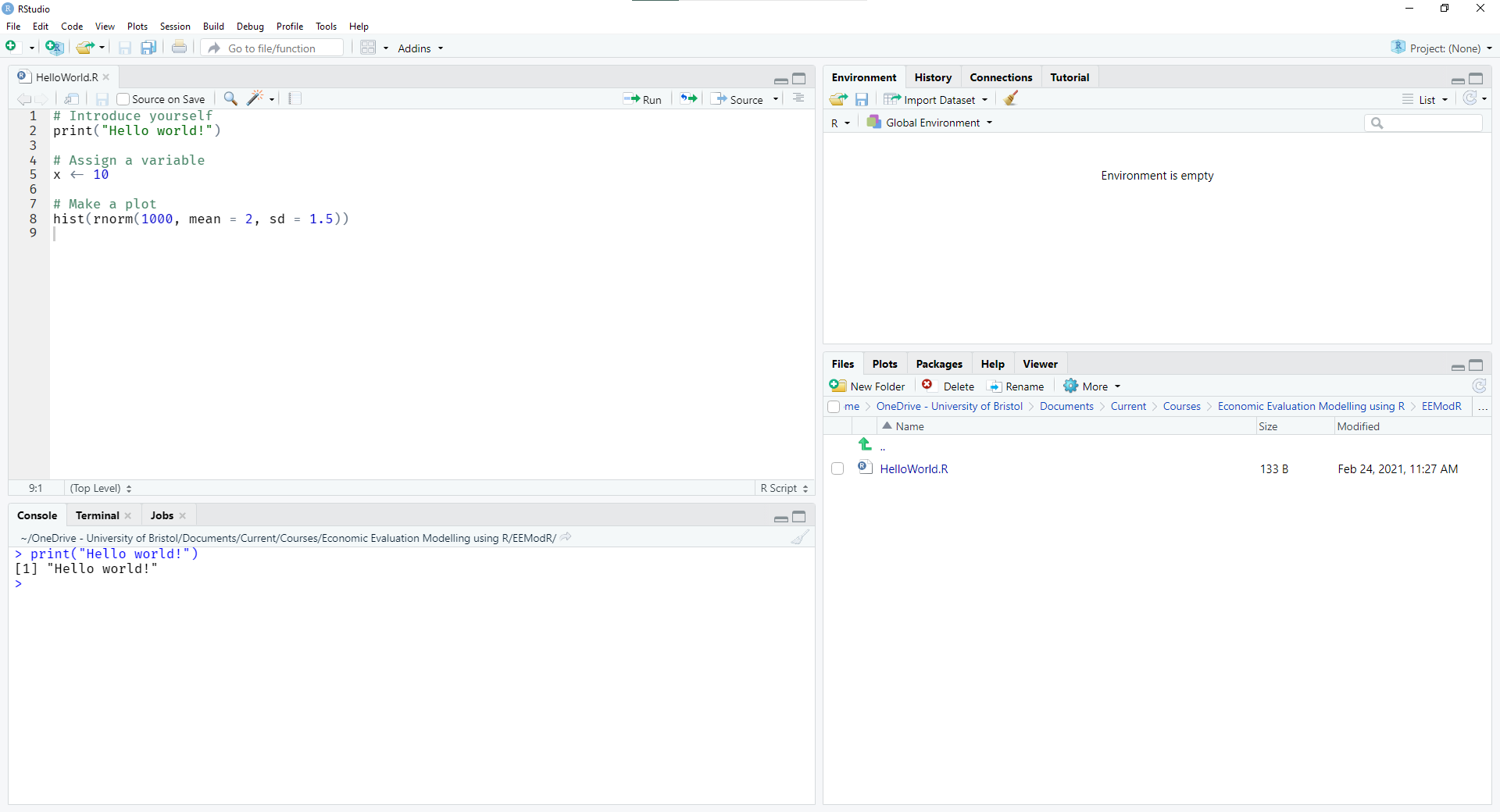
Figure 2.1: The Rstudio graphical interface

You can type and run commands directly in the console pane (bottom left). Once a command is typed in, you press Enter to run it. It is also possible to use Tab to autocomplete commands. Output from a script (see shortly) is also displayed in this console area. A useful feature is that you can scroll back through previous commands with the arrow keys.

Scripts with a saved sequence of R commands are displayed in the source pane (top left). You can create a new script with File > New Script or the button. R scripts usually have the extension .R or .r. One or more lines of the script can be run by putting the cursor on the line or highlighting multiple lines, and then pressing the keyboard shortcut Ctrl + Enter (on Windows and Linux; Cmd + Return on Mac) or the button.

The environment pane (top right) shows objects that are currently available, such as variables, data frames, and user-defined functions.

In the bottom right of the interface are tabs for the plot pane, help pane and files pane. In the bottom right of Figure 2.1 is currently the file pane, which allows you to access files and open scripts. By default, this opens to your current working directory. Clicking the other tab headers will open the plot and help panes. These will automatically open if you run a plot or help command, respectively.

2.2.1 Projects

When organising an analysis or developing a model, you may have lots of files within a project folder, including data, multiple analysis scripts, and output figures and tables. Rstudio has a feature called projects that is designed with this in mind. These automatically open the file browser to your project directory, opens up the files you last used in the source pane, and sets your working directory.

Working directories

The worst approach to setting working directories is to use absolute paths when loading data or calling source scripts

• read.csv("C:/Users/UserX/Documents/Projects/BigAnalysis7/data/raw.csv")
• png(file = "C:/Users/UserY/Documents/Projects/BigAnalysis7/figures/CEAC.png")

If another analyst wanted to rerun such a script, they would fist need to save all necessary files, then take note of the new locations, and finally change all these absolute paths to the new locations. This is not only time consuming but also prone to error.

The not so bad approach is to use setwd() and relative paths

• setwd("C:/Users/UserX/Documents/Projects/BigAnalysis7/R")
• read.csv("../data/raw.csv")
• png(file = "./figures/CEAC.png")

Using this approach, the second analyst could copy the entirety of the necessary folders (e.g. data and figures in the above approach) to some new root directory, and then only change the directory in setwd() to to this new directory. However, this still relies on manual manipulation of working directories and correct copying/sharing of necessary folders.

The best approach is perhaps to use an Rstudio project, which automatically sets the correct working directory. Using this approach a user would open the project file BigAnalysis7.Rproj, saved in the main project directory that contains all the necessary subfolders, scripts, and data, and then use relative paths

• read.csv("../data/raw.csv")
• png(file = "./figures/CEAC.png")

possibly in combination with suitable packages (e.g. here; see Section 2.3.5 for more details on installing packages).

R paths

Paths in R are specified with forward slashes /, following the Unix notation.

Creating and opening projects

The project switcher in the top right lets you create a new project or switch to recent projects.

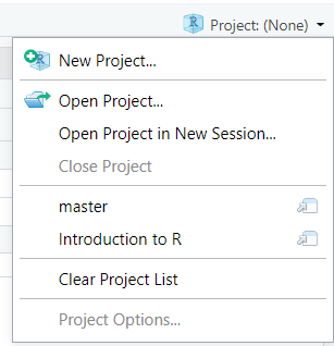
You can also create/open projects via the File menu, or the button in the toolbar. Double-clicking on an .Rproj file in explorer will also open the project in Rstudio.

Save Workspace?

When you close Rstudio, you may get a message asking you whether you want to save your workspace:

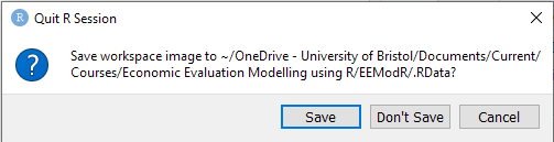
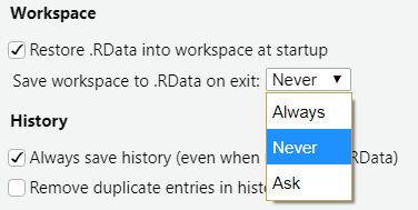
We strongly recommend that you choose Don’t save. Saving your workspace is not reproducible: future results will depend on previously run code, and It is easy to introduce hidden errors or lose work. You can disable this option permanently by going to Tools > Global Options and choosing Save workspace to .RData on exit: Never

2.3 Basic operations

We start our discussion of the R language with the very basics: standard mathematical operations, character strings, assigning variables, and special values in R.

2.3.1 Maths

In R, the order of operations follows the usual “Brackets Order Division Multiplication Addition Subtraction” (BODMAS) rules

3 * 3 + 3

[1] 12

(4 - 3) / 3

[1] 0.3333333

2^10 - 1

[1] 1023

Many common mathematical functions are available as built-in functions, including natural logarithms (log()), natural exponent (exp()), and square roots (sqrt()). These are called by passing an argument to the function, for example as in the following code.

sqrt(9)

[1] 3

2.3.2 Strings

Character strings are surrounded by double " or single ' quotes, as in the following.

"Hello world!"

[1] "Hello world!"

'Welcome'

[1] "Welcome"

Later in this chapter we will cover some basic functions for manipulating strings.

2.3.3 Assignment

So far we have only printed out the results of an expression to the console. To save the results from a command, to be accessed later or for further manipulation, we can assign a variable using the assignment arrow operator <-

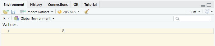
x <- 2^3

This assigns the result of 2^3 to the variable x; you will notice that this is now visible in the environment pane in the top-right of Rstudio.

The value of any variable can be printed to the console using the print() function, or simply by typing the name of the variable

print(x)

[1] 8

x

[1] 8

A variable can be used in expressions or functions

x * 10

[1] 80

sqrt(x)

[1] 2.828427

Any object in R can be assigned to a variable: simple numeric values or character strings; data structures like vectors (Section 2.4.1), matrices (Section 2.4.3), lists (Section 2.8.1), or data frames (Section 2.8.2); or results from a model function like glm(). Valid variable names must start with a letter, and can only include letters (case-sensitive), symbols such as “_” or “.” or numbers.

Descriptive variable names make code much easier to read and follow. It is not clear what the following code is for:

x1 <- 20000
x2 <- 0.2
x3 <- 1800
x4 <- x2 * x1 - x3

This is much better:

threshold <- 20000
qualy <- 0.2
cost <- 1800
net_benefit <- qualy * threshold - cost

2.3.4 Special values

There are several special values built-in to R. Missing values (see Chapter 6) are indicated by NA.

NA + 1

[1] NA

Infinite values are Inf or -Inf.

2 / 0

[1] Inf

log(0)

[1] -Inf

Sometimes the result of a calculation is undefined (not a number) NaN.

log(-1)

[1] NaN

You may also come across NULL, which is an empty value (length zero).

2.3.5 Installing and loading packages

Packages are collections of related functions, data, help files, and examples. We can load a built-in, or already installed, package using the library() command.

library(survival)

There is a whole universe of user-created R packages that can be installed and loaded, many of which are encountered in this book. These include dplyr, tidyr, and data.table for working with data; ggplot2 a “grammar of graphics” for creating plots; metafor, gemtc, and multinma for meta-analysis; and BCEA, heemod, and hesim for health economic modelling. Many packages can be installed from the Comprehensive R Archive Network (CRAN) directly within an R session using install.packages().

install.packages("BCEA")

Once installed, the package can be loaded using library(). Packages only need to be installed once but need to be loaded for each session of R. Packages can be updated and to do this it is best to use the Tools > Check for Package Updates menu in Rstudio or the update.packages() function.

2.4 Types of variables

2.4.1 Vectors

Vectors are ordered sets of values of the same type, constructed using the “combine” operator, c().

c(2, 6, 3, 1)

[1] 2 6 3 1

c("Apple", "Orange", "Banana")

[1] "Apple"  "Orange" "Banana"

costA <- 12.50 # A named numeric variable with value 12.50
costB <- 25
costC <- 61.80
c(costA, costB, costC)

[1] 12.5 25.0 61.8

Note

The # is the comment symbol, the remainder of the line is ignored

The length() function returns the length of the vector (the number of elements).

length(c(costA, costB, costC))

[1] 3

Sequences and repeating values

We can use the “:” operator or seq() function to create sequences.

1:5

[1] 1 2 3 4 5

seq(from = -20, to = 30, by = 10)

[1] -20 -10   0  10  20  30

We can also use rep(), with arguments times and each to create vectors by repeating values

rep(2, times = 3)

[1] 2 2 2

rep(1:3, times = 2)

[1] 1 2 3 1 2 3

rep(1:3, each = 2)

[1] 1 1 2 2 3 3

Help

Find help for a function using ?, for example ?rep. You can also type help(name_of_the_function) or even more specifically help(name_of_the_function, package = "name_of_the_package_it_belongs_to").

Named vectors

Elements of vectors can be named at creation, or we can use the names() function to get/set names of a vector.

costs <- c(A = costA, B = costB, C = costC)
costs

   A    B    C 
12.5 25.0 61.8 

names(costs)

[1] "A" "B" "C"

names(costs) <- c("costA", "costB", "costC")
costs

costA costB costC 
 12.5  25.0  61.8 

It is a good idea to give the elements of vectors meaningful names. This will avoid the error of someone trying to access the wrong element; e.g. it is better and less error-prone to access prices["orange"] to get the price of an orange instead of prices[3].

Indexing and subsetting

Vectors can be indexed by position or name using square brackets [], and multiple elements can be returned by indexing with a vector. The combine operator c() can be used to create an indexing vector.

costs[2]

costB 
   25 

costs["costB"]

costB 
   25 

costs[c(1, 3)] 

costA costC 
 12.5  61.8 

costs[c("costA", "costC")]

costA costC 
 12.5  61.8 

Vectors can be subset with a logical vector of boolean values.

costs > 20

costA costB costC 
FALSE  TRUE  TRUE 

costs[costs > 20]

costB costC 
 25.0  61.8 

costs[costs != 25]

costA costC 
 12.5  61.8 

We can also use indexing to replace the values of vector elements. Place square brackets [] on the left-hand side of an assignment <- to replace selected values.

costs[1] <- 10
costs

costA costB costC 
 10.0  25.0  61.8 

costs[2:3] <- c(20, 30)
costs

costA costB costC 
   10    20    30 

Vector operations

Operations can be applied across every element in a vector at once.

costs + 100

costA costB costC 
  110   120   130 

exp(1:5)

[1]   2.718282   7.389056  20.085537  54.598150 148.413159

Operations can also involve more than one vector.

costs + c(100, 200, 300)

costA costB costC 
  110   220   330 

costs * 1:3

costA costB costC 
   10    40    90 

Vectors of different lengths will be recycled to match the longest.

costs * 1:2

costA costB costC 
   10    40    30 

So in the case above, because costs has 3 values but 1:2 only has two, the elements of costs are multiplied as cost[1]*1, cost[2]*2 and cost[3]*1 — this example shows how recycling can lead to hidden mistakes and so care is needed when using it.

2.4.2 Strings

Character strings and functions for their manipulation are a useful feature in R. Not only do they allow natural naming and indexing of other data types, they also facilitate the analysis and exploration of text data.

R can join strings together using the paste() function, which takes any number of strings as arguments. You can provide the optional argument sep to say what string separator to put between the joined strings.

paste("A", "B", "C")

[1] "A B C"

paste("A", "B", "C", sep = ",")

[1] "A,B,C"

paste0("A", "B", "C")               # Equivalent to sep = ""

[1] "ABC"

The paste() function also works on vectors and can combine vectors with other vectors or with scalars (single element vectors). The collapse argument collapses string vectors into a single string.

abc <- c("a", "b", "c")
paste(abc)

[1] "a" "b" "c"

paste("Letter", abc, sep = "-")

[1] "Letter-a" "Letter-b" "Letter-c"

paste("Letter", abc, sep = "-", collapse = ", ")

[1] "Letter-a, Letter-b, Letter-c"

paste(1:5, abc)

[1] "1 a" "2 b" "3 c" "4 a" "5 b"

For example, this functionality could be used to create a unique identifier out of patients’ initials, age, and gender.

2.4.3 Matrices

Vectors are one dimensional objects, e.g. \[(1,~2,~3,~4)\] while matrices are two dimensional objects, for instance \[\begin{pmatrix} 1 & 2 \\ 3 & 4 \end{pmatrix}.\] R has a powerful suite of matrix functions, which are very useful for Markov or multistate modelling in HTA (see Chapter 9 and Chapter 11). Matrices are created using the matrix() function which takes arguments for the data, number of rows nrow and number of columns ncol. If no data are supplied, the matrix is filled with NA.

matrix(nrow = 2, ncol = 3)

     [,1] [,2] [,3]
[1,]   NA   NA   NA
[2,]   NA   NA   NA

matrix(1:6, nrow = 2, ncol = 3) # The vector 1:6 is the data argument

     [,1] [,2] [,3]
[1,]    1    3    5
[2,]    2    4    6

Note that R works in “column-major” order — the numbers in the data 1:6 are filled by columns, by default. This behaviour can be overruled by specifying the option byrow=TRUE.

matrix(1:6, nrow = 2, ncol = 3, byrow = TRUE)

     [,1] [,2] [,3]
[1,]    1    2    3
[2,]    4    5    6

Note

Arguments passed to R functions do not need to be named, so long as they are in the correct order.

We can return the dimensions (number of rows, number of columns) of a matrix using dim(), or the number of rows and columns using the built-in functions nrow() and ncol(). The length() function returns the number of elements — not the number of rows!

(m <- matrix(1:6, ncol = 3))

     [,1] [,2] [,3]
[1,]    1    3    5
[2,]    2    4    6

(note here that placing parentheses () around an expression prints the output to the console).

dim(m)

[1] 2 3

nrow(m)

[1] 2

ncol(m)

[1] 3

Indexing, subsetting, assignment, and naming

Index of matrices works just like vector indexing, subsetting, and assignment — but now with two dimensions rows, columns.

m[1, 2]          # First row, second column

[1] 3

m[2, 2:3]        # Second row, columns 2 and 3, and It is now a vector!

[1] 4 6

m[2, ] <- 10:12  # Replace second row
m

     [,1] [,2] [,3]
[1,]    1    3    5
[2,]   10   11   12

When indexing or subsetting a matrix, unnecessary dimensions are dropped by default. The result is then a vector rather than a matrix. This can cause trouble if your code is designed only for matrices (e.g., calling the dim() argument on a vector would return NULL rather than the number of elements, giving a potential error). This behaviour can be changed using the drop = FALSE argument.

m[1, , drop = FALSE]   # First row but still a matrix

     [,1] [,2] [,3]
[1,]    1    3    5

m[, 3, drop = FALSE]   # Third column but still a matrix

     [,1]
[1,]    5
[2,]   12

m[1, 2, drop = FALSE]  # A 1x1 matrix

     [,1]
[1,]    3

Just like a vector can have named elements, matrix rows and columns can also have names. These are set and accessed using the rownames() and colnames() functions. As with accessing vectors, it is safer to use meaningful names to subset a matrix, to avoid errors when remembering which is which element of each dimension.

colnames(m) <- c("A", "B", "C")
rownames(m) <- c("cost", "qaly")
m

      A  B  C
cost  1  3  5
qaly 10 11 12

colnames(m)

[1] "A" "B" "C"

rownames(m)

[1] "cost" "qaly"

m["qaly", ]

 A  B  C 
10 11 12 

Element-wise operations

Operations can be applied across every element in a matrix at once.

(m2 <- matrix(1:4, nrow = 2))

     [,1] [,2]
[1,]    1    3
[2,]    2    4

m2 + 100

     [,1] [,2]
[1,]  101  103
[2,]  102  104

exp(m2)

         [,1]     [,2]
[1,] 2.718282 20.08554
[2,] 7.389056 54.59815

Matrices may also be added together, with corresponding elements added, as long as they are the same dimension. If the dimensions are different R will give an error.

m2 + m2

     [,1] [,2]
[1,]    2    6
[2,]    4    8

(m3 <- matrix(1:6, ncol = 3))

     [,1] [,2] [,3]
[1,]    1    3    5
[2,]    2    4    6

m2 + m3

Error in m2 + m3: non-conformable arrays

The same applies to element-wise multiplication or division. R will multiply or divide corresponding elements if the matrices have the same dimensions, and give an error if not.

m2 * m2

     [,1] [,2]
[1,]    1    9
[2,]    4   16

m2 * m3

Error in m2 * m3: non-conformable arrays

Matrix multiplication

Multiplying two matrices \(A \times B\) means taking the sum-product of every row of \(A\) with every column of \(B\) (see Section 4.6)

\[A = \begin{pmatrix} 2 & 3 \\ 2 & 1 \end{pmatrix} \qquad B = \begin{pmatrix} 2 & 3 & 1 \\ 0 & 3 & 3 \end{pmatrix}\]

\[A \times B = \begin{pmatrix} 4 & 15 & 11 \\ 4 & 9 & 5 \end{pmatrix}.\]

Matrix dimensions must be compatible, and order matters: (rows, columns)(rows, columns) = (rows, columns). For example, \(B \times A\) is not possible here, since ncol(B) does not equal nrow(A). Matrix multiplication in R uses the “%*%” operator and gives an error if the dimensions are not compatible.

m2 %*% m2

     [,1] [,2]
[1,]    7   15
[2,]   10   22

m2 %*% m3

     [,1] [,2] [,3]
[1,]    7   15   23
[2,]   10   22   34

m3 %*% m2

Error in m3 %*% m2: non-conformable arguments

Other matrix operations

Transposing a matrix (written \(A^\top\); see Section 4.6.2.2) means switching the rows and columns. This is implemented in R through the t() function.

t(m2)

     [,1] [,2]
[1,]    1    2
[2,]    3    4

Inverting a square matrix (written \(A^{-1}\) — see again Section 4.6.2.2) means solving \[A \times A^{-1} = A^{-1} \times A = I\] where \(I\) is the identity matrix (a matrix with 1s on the diagonal and 0s everywhere else). This is implemented using the solve() function.

m2_inverse <- solve(m2)
m2_inverse %*% m2

     [,1] [,2]
[1,]    1    0
[2,]    0    1

Matrices of compatible sizes can be joined together by rows using the rbind() function, or by columns using the cbind() function. These functions take any number of compatible matrices as their arguments.

cbind(m2, m3)

     [,1] [,2] [,3] [,4] [,5]
[1,]    1    3    1    3    5
[2,]    2    4    2    4    6

rbind(m2, m2)

     [,1] [,2]
[1,]    1    3
[2,]    2    4
[3,]    1    3
[4,]    2    4

2.5 For loops

The for statement is an example of a control flow structure, which allow us to alter the usual sequential flow of commands through a program. For loops are used to perform an action or actions over a sequence of values.

for (i in 1:3) {
  print(i)
}

[1] 1
[1] 2
[1] 3

The general syntax of a for loop follows the structure

output 
for (var in sequence) {
  body
}

We pre-allocate any output (e.g., a vector or matrix), rather than growing it in size as we progress through the loop; this is important for efficiency, as repeatedly growing an object can be very slow. var is a variable that will be updated with each value of sequence in turn. sequence is the vector to loop over, e.g. 1:10 or 1:nrow(X) or c("Apple", "Pear", "Orange"). body is code that will be executed for each element of sequence.

A less trivial example is provided below, which uses vector and matrix multiplication to simulate from a simple cohort Markov model (Chapter 9).

P <- matrix(c(0.75, 0, 0.25, 1), ncol = 2) # The transition matrix
P

     [,1] [,2]
[1,] 0.75 0.25
[2,] 0.00 1.00

# Matrix to store state occupancy at each of 4 cycles
state <- matrix(nrow = 4, ncol = 2) 
state[1, ] <- c(1, 0)  #  Initial state

for (i in 2:nrow(state)) {
  state[i, ] <- state[i - 1,] %*% P # Markov update
}

state

         [,1]     [,2]
[1,] 1.000000 0.000000
[2,] 0.750000 0.250000
[3,] 0.562500 0.437500
[4,] 0.421875 0.578125

2.6 Distributions and generating samples

R was designed for statistical analysis, so it is unsurprising that it has a wealth of built-in functionality for statistical distributions. These functions are of the form

• ddist(x,args) the density function at value x
• pdist(q,args) the cumulative distribution function (CDF) at quantile q
• qdist(p,args) the inverse CDF / quantile function at probability p
• rdist(n,args) generating random samples of size n

where dist is the short name of a distribution, e.g. norm, gamma, beta, or unif for a Normal, Gamma, Beta or Uniform distribution, respectively; and args includes the parameters of the distribution, e.g. mean = 0, sd = 1. See Section 4.3 for more discussion on probability distributions. For a full list of the built-in distributions see ?distributions

The rdist functions are used to generate random samples from distributions. For example, these can be used these to introduce uncertainty about model parameters.

x1 <- rnorm(n = 1000, mean = 0, sd = 1)
head(x1)

[1]  0.01874617 -0.18425254 -1.37133055 -0.59916772  0.29454513  0.38979430

hist(x1)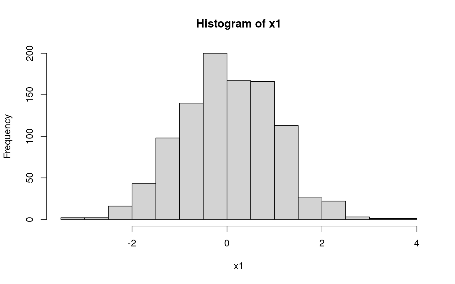

The algorithm for random number generation is initialised from a seed value. It is good practice to set the seed value at the beginning of an analysis script.

set.seed(22032021)

This ensures that results, even if using random samples, are reproducible.

rnorm(4)

[1] -0.124689279 -0.881238700  0.003229584 -0.653726718

rnorm(4)

[1] -0.110203087  1.103632036 -0.484763152 -0.005375358

set.seed(22032021)
rnorm(4)

[1] -0.124689279 -0.881238700  0.003229584 -0.653726718

2.7 Saving graphical outputs

2.7.1 Saving plots from the plot window

Rstudio provides a simple point-and-click process for saving plots.

1. Click the export button in the plot window, then Save as Image

2. In the pop-up window, specify the image format, output directory and file name, set image dimensions, and hit Save

The Save as PDF and Copy to Clipboard options work in much the same way.

2.7.2 Using graphics devices

A disadvantage of using the Rstudio interface to save plots is that it needs to be done manually for each plot. This can be very time consuming if running an analysis with many outputs (e.g., sensitivities, subgroups, secondary outcomes, etc.). It also prevents analyses from being reproducible, as it will not be clear which plots were saved and with what names. A more reproducible and automated approach is to use a graphics device.

device(filename="myplot.png", options)
plot code
dev.off()

You first open a graphics device using a device(), e.g. png(), pdf(), tiff(), with options such as width and height to specify the dimensions in units (e.g. pixels "px" or inches "in") and res to specify the resolution for raster devices like png(). The default resolution is 72 but 300 or higher is best for publications, or to use a vector device such as pdf(). With the device open, you run your plot code, such as plot() or hist(). Finally, you close the device with dev.off() to write the output to the file.

An example of this process is below, which plots a histogram with beta distribution curve to file named "logRR_histogram.png".

png("./figures/logRR_histogram.png", width = 7, height = 5, 
    units = "in", res = 300)

hist(bl_risk, breaks = 50, freq = FALSE)
curve(dbeta(x, 98, 402 - 98), add = TRUE, col = "darkred")

dev.off()

Even more efficiently, we can make use of tools such as rmarkdown (Xie et al., 2018) or quarto (Allaire et al., 2024), which allow you to write a single document containing plain-language description and R “chunks” of code, which get executed at compilation time. The resulting output is then embedded in the compiled document (in html, pdf, docx or other formats).

2.8 Data types

R has a wide range of data types that serve different but overlapping purposes. We have encountered some common data types. Scalar variables are single values, so of length 1. They can be numeric, character, or logical. Vectors are one-dimensional sets of the same basic type created using the collation function c(). Matrices are two-dimensional sets of the same basic type created using the matrix() function. We will now introduce three more: lists, data frames, and arrays

2.8.1 Lists

Lists are the most general type of data structure. Their elements can be any other data type, including vectors, data frames, matrices, and other lists. There is also no requirement for elements to be the same length or even the same type. This flexibility makes them useful for returning output from functions.

They are created using the list() function

list(x1 = value1, x2 = value1, x3, x4)

Each of the arguments specifies one element, in order of appearance, as either a named element:

• x1 = value1 creates an element named x1 with values from value1
• x2 = value2 creates an element named x2 with values from value2

Or unnamed elements

• x3 creates an unnamed element from object x3
• x4 creates an unnamed element from object x4

For example, we can define a list with one numeric, one string, one vector, and one (empty) list element

l <- list(one = 1, "two", three = 3:6, list())

Lists can be indexed and subset by position or name (if named).

l[3]

$three
[1] 3 4 5 6

l[c("one", "three")]

$one
[1] 1

$three
[1] 3 4 5 6

l[["three"]]

[1] 3 4 5 6

l$three

[1] 3 4 5 6

There are some notable differences between the extraction operators above. The [ operator returns a list (think container and contents) and can select multiple elements. The [[ operator returns an element (think contents only) and can can only select one element. The $ operator is a shortcut for [[. Names can be shortened for $ (e.g., l$th) but this is not recommended. An advantage of [[ is that element names can be passed as variables.

named_element <- "three"
l[[named_element]]

[1] 3 4 5 6

This feature can be useful for scripting or programming, for example to select certain elements based on user input.

2.8.2 Data frames

Data frames are the standard way of storing rectangular data. This type of data is in a format where there are rows of records (e.g. individuals in a trial) and columns of variables (e.g. ID, age, smoking status, outcome):

ID	Age	Smoke	Outcome
1	39	Never	FALSE
2	45	Former	TRUE
3	36	Never	TRUE
4	52	Current	TRUE
…	…	…	…

Earlier we discussed matrices, which are another way of storing rectangular data: all rows are the same length and all columns are the same length. Data frames are more flexible in that they can have columns with different types (e.g. numeric, character, logical), whereas an entire matrix must be the same type. In a data frame, the rows are always records or observations, but a matrix makes no distinction between rows and columns. Unlike data frames, matrices allow matrix multiplications which are computationally very efficient.

Note

Behind the scenes, a matrix is implemented as vector with a dimension property or “attribute”, whereas a data frame is implemented as a list of vectors.

In R, you can construct a data frame using the data.frame() function

data.frame(x1 = value1, x2 = value2, x3, x4)

Each of the arguments specifies one column, in order of appearance, either as a name-value pair:

• x1 = value1 creates column x1 with values from value1
• x2 = value2 creates column x2 with values from value2

or just object names:

• x3 creates column x3 from object x3
• x4 creates column x4 from object x4

A more structured example is the following.

id <- 1:4
x2 <- c(39, 45, 36, 52)
smoking <- data.frame(
  id,
  age = x2,
  smoke = c("Never", "Former", "Never", "Current"),
  outcome = c(FALSE, TRUE, TRUE, TRUE)
)
smoking

  id age   smoke outcome
1  1  39   Never   FALSE
2  2  45  Former    TRUE
3  3  36   Never    TRUE
4  4  52 Current    TRUE

Indexing and subsetting is very similar to matrices with [rows, columns].

smoking[2:3, c("id", "age")]     # Rows 2-3, columns id and age

  id age
2  2  45
3  3  36

Columns can also be selected directly, like elements of a list. Notice that there are no commas separating dimensions in the example below.

smoking[c("id", "age")]  # return a data frame, select multiple columns

  id age
1  1  39
2  2  45
3  3  36
4  4  52

smoking[["age"]]         # return a vector, can only select one column

[1] 39 45 36 52

smoking$age              # shortcut for `[[`

[1] 39 45 36 52

2.8.3 Arrays

Arrays extend matrices to more than two dimensions. For example a 3D array storing the state occupancy matrix for multiple treatments across cycles in a Markov model (Chapter 9) might have dimensions [cycle, treatment, state]. Like matrices, elements of an array must all be the same data type (e.g., numeric or character). Furthermore, arrays allow matrix multiplications on two-dimensional sub-matrices or one-dimension sub-vectors.

Arrays are constructed using the array() function.

array(data = data, dim=dim, dimnames = dimnames)

where:

• data is a vector of data to fill the array (or NA)
• dim is an integer vector giving the size in each dimension
• dimnames is an (optional) list of character vectors giving the names of the dimensions.

The elements of an array can be accessed using the [ operator in exactly the same way as a matrix — just with more dimensions.

Here we create a 3-dimensional array for storing the occupancy matrix for a Markov model. This has dimensions for treatments, states, and cycles. There are 2 treatments (A, B), 2 states (healthy, ill), and 3 cycles, which define the number of elements of each dimension.

array(
  dim = c(3, 2, 2),
  dimnames = list(
    cycle = NULL, treatment = c("A", "B"), state = c("Healthy", "Ill")
  )
)

, , state = Healthy

      treatment
cycle   A  B
  [1,] NA NA
  [2,] NA NA
  [3,] NA NA

, , state = Ill

      treatment
cycle   A  B
  [1,] NA NA
  [2,] NA NA
  [3,] NA NA

Applying functions to dimensions of an array

Sometimes we need to apply a function over the dimensions of an array or matrix. We can use the apply() function to do this, with the following syntax:

apply(X, MARGIN, FUN, ...)

• X is the input array or matrix

• MARGIN is the dimension/dimensions to apply over (e.g. with a matrix 1 for rows, 2 for columns)

• FUN is the function to apply, as a bare function name or character string

• ... are additional arguments passed to the function FUN

For example, we can sum each row in a matrix or calculate the mean of each column.

m <- matrix(1:6, ncol = 3)
m

     [,1] [,2] [,3]
[1,]    1    3    5
[2,]    2    4    6

apply(m, 1, sum)

[1]  9 12

apply(m, 2, mean)

[1] 1.5 3.5 5.5

Tip

The rowSums(), colSums() and rowMeans(), colMeans() functions are convenient shortcuts for these common uses of apply(), and are also slightly more efficient.

2.8.4 Converting between data types

Data can be coerced from one type to another using the as.type() functions, where type is the data type to which you want to convert. Examples include as.matrix(), as.data.frame(), and as.list().

(m <- matrix(1:6, ncol = 2, dimnames = list(NULL, c("x1", "x2"))))

     x1 x2
[1,]  1  4
[2,]  2  5
[3,]  3  6

(df <- as.data.frame(m))

  x1 x2
1  1  4
2  2  5
3  3  6

(l <- as.list(df))

$x1
[1] 1 2 3

$x2
[1] 4 5 6

2.9 Importing and exporting data

R has functionality to read data in a variety of formats, including that output by other software such as Excel, STATA, and SAS. It also has functionality for saving data in different formats, including in an efficient format that is only readable by R. In this section we discuss access to the most commonly used formats.

2.9.1 Reading and writing CSV files

The CSV (comma separated value) format is a very common way of sharing data with other people or software packages as it is readable by most statistical and data management software. This includes Microsoft Excel.

trt,cost_direct,cost_community,
"A",1701,1055,
"B",1774,1278,
"C",6948,2059,

The syntax is

object <- read.csv(file)

to read a CSV file into a data frame object, and

write.csv(object, file=file)

to write a data frame/matrix object to a named file.

Tip

The read.table() and write.table() functions provide even more control over the input/output format, e.g. using tabs as separators instead of commas.

2.9.2 Reading and writing Excel files

You can also read and write Excel spreadsheets directly without converting to CSV. There are a few different packages that will do this, here we use readxl and writexl.

install.packages("readxl")
install.packages("writexl")
library(readxl)
library(writexl)

To read an Excel file, the basic command from the readxl package is

object <- read_excel(file, sheet = sheet, range = range)

This reads the Excel file file into a data frame object, taking data from the range of cells range on sheet sheet. If sheet is omitted, the first sheet will be used. If range is omitted, the range of cells will be guessed. Further options include controlling column names and types, skipping rows.

Writing Excel files

To write an Excel file using the writexl package, the command is

write_xlsx(object, file = file)

This writes a data frame object to an XLSX file. Pass a named list of data frames as object to create multiple sheets.

The openxlsx package provides more control in writing and styling Excel spreadsheets, and is worth investigating if this functionality would be of use. The xlsx package is another but requires Java, which limits compatibility. The googlesheets4 package serves a similar purpose for working with Google Sheets.

2.9.3 Saving and loading R objects

It can sometimes be useful to save, and later load, an R object. For example you may want to save the output from a model or script if it takes a long time to compute, like the results from a large probabilistic Markov model (Chapter 11) or complex network meta-analysis (Chapter 10). This also aids with sharing code and ensuring analyses are reproducible. The probabilistic samples could be saved to your R project and collaborators could run their own post-processing code.

R objects are saved and loaded using the functions saveRDS() and readRDS(), respectively.

saveRDS(object, file = file)
object <- readRDS(file)

where object is the object to save and file is the file path to save to (usually with extension .rds).

There are also functions save() and load(), which allow you to save and load multiple objects at once. However we do not recommend these, as load() in particular is less explicit and can easily lead to overwriting objects in your current environment.

2.10 Functions and control flow

Controlling program flow is an important feature of R when writing complex programs. We often want to choose whether code runs or not, depending on some condition. For example, applying certain costs only in the first cycle of a model, or including an event disutility only when running a sensitivity analysis. We can achieve this using if, else if and else statements, for example in the following form.

if (condition1) {
  expression1
} elseif {condition2} {
  expression2
} else {
  expression3
}

This means that if condition1 is TRUE, then run the code expressions1. Otherwise, if condition2 is TRUE, run the code expressions2. It neither of these conditions is TRUE, run the code expressions3.

Once a condition is met, no further conditions or expressions are evaluated. You may have as many else if statements as you like, or none at all. You may only have one else statement, or again none at all. Each condition must be of length 1, i.e. it must evaluate to a single TRUE or FALSE.

2.10.1 Logical conditions

We have already met some of the comparison operators:

• == equals
• != not equals
• < less than
• <= less than or equal to
• > greater than
• >= greater than or equal to

All of these can be used to define conditions in if statements.

x <- 5
if (x > 1) {
  print("Greater than 1")
} else {
  print("Less than or equal to 1")
}

[1] "Greater than 1"

Other useful functions that return logical values include

• is.na(), is.infinite(), is.null() to check whether a value is missing, infinite, or NULL

• %in% checks whether a value is in a set, e.g. x %in% 1:5 or
  trt %in% c("B", "C")

• any() and all() check whether any or all of a set of conditions are met, e.g. any(is.na(x))

Multiple logical conditions can be combined with || (OR) and && (AND).

x <- 5
y <- 3
(x > 1) || (y > 4)

[1] TRUE

These || and && are “lazy” in that they will not evaluate every condition if it is not necessary; they evaluate conditions from left to right, and stop when the overall result is determined.

(x > 1) || (z > 0)  # || and && are lazy - z does not exist

[1] TRUE

There are also “single” versions | and &. These operate on and return logical vectors. These are not “lazy” as every condition is always evaluated. For an if statement, you should always use the “double” versions || and && as a single logical result is needed. Finally, any logical statement can be negated using !, e.g. !(x > 2).

2.10.2 Functions

Functions are the essential building blocks of modular and reusable code. The same code can be reused multiple times, without copying and pasting or repetition. This modular approach gives fewer opportunities for mistakes as the code only needs to be correct once, rather than each time it is repeated. It also make it easier to debug, maintain, and update, as this needs to be done only once rather than each place the function is used. Modular code with descriptive function names can be easier to follow, for example generate_input_parameters(), generate_net_benefit(), or plot_ceac(). Finally, modularisation eases collaboration as user X can utilize a function developed by user Y, and user Y can continue to maintain and improve the shared function.

A guiding principle is that if you copy and paste code more than twice, you should consider making a function instead.

Functions are created with the following syntax

fn <- function(arguments) {
  body
  return(out)
}

This creates a function called fn that takes inputs arguments. Arguments may have default values like discount = 3.5 or threshold = 20000, or can be left without default values like n_samples or costs. The function runs the code in the body of the function, and then exits by returning the object out, for example, a vector or list. Note that if the return() statement is omitted, the result of the last evaluated expression in body will be returned. We recommend always using return() to avoid ambiguity and make it explicit what the output of a function is. Once the lines above are executed by R, the function can be called as fn(arguments).

A simple example is a function to calculate the logit transform (see Equation 4.26).

logit <- function(x) {
  return(log(x / (1 - x)))
}

logit(0.5)

[1] 0

Another example is a function to calculate net benefit given cost, QALY, and threshold (with a default threshold value of 20000).

net_benefit <- function(qaly, cost, threshold = 20000) {
  return(threshold * qaly - cost)
}

net_benefit(qaly = 0.8, cost = 1875)

[1] 14125

net_benefit(0.8, 1875, threshold = 10000)

[1] 6125

An important concept when using functions in R is variable scope. Variables created within a function are local to that function. They cannot be accessed outside of the body of the function and they do not change variables in the global environment (i.e., the values in the Environment Pane).

x <- 10

f <- function(value) {
  x <- value
  return(x)
}

f(5)

[1] 5

x

[1] 10

Within a function you can also access global variables but this is not good practice as it limits reusability and reproducibility. Firstly, the function would not be self-contained, and thus not easily reusable, if it was dependent on certain global variables being defined. Secondly, the output would depend on the current state of the global environment, limiting reproducibility.

Functions can do more than just compute and return values. To aid with more complex functions, we can use the stop() function to halt function execution immediately and raise an error message.

This is very useful for checking that function arguments are valid, and giving an informative error message otherwise:

if (threshold <= 0) {
  stop("threshold must be positive")
}

The warning() function raises a warning message, but continues execution. In most cases, it would be better to use stop() if the function has been passed incorrect arguments. The message() function prints a message to the console, for example to inform the user of progress in a long-running function.

As your function become longer there is an increased need for debugging. To aid in this purpose, you can use print() or cat() to output calculation steps to the console.

A much more powerful option is to use the debugging tools built-in to R and Rstudio. If you run debugonce(fun) before calling the function fun, you can “step inside” the function whilst it runs and investigate line-by-line. Alternatively, place a call to browser() in your function at the line where you want to “step in”. The debugged function will be opened in the source pane, and the line that will be executed next by R is highlighted:

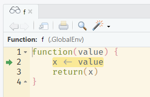
You can then use the console to investigate and run commands within the current state of the function environment, for example to print the current values of variables or to evaluate pieces of code. Rstudio provides buttons above the console pane to control the debugger.

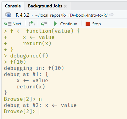
From left to right, these buttons:

• Run the currently highlighted line, and move to the next
• If a function is to be called on the highlighted line, step inside this function with the debugger
• Run the remainder of a loop or function
• Continue running the remainder of the function until it exits, or until another browser() break point is reached
• Stop running the function immediately

2.11 Final remarks

This has been a rapid tour of the functionality of R. If you have experimented while reading, you should be sufficiently familiar with R to manage the remainder of this book. Even if you encounter a topic we have not discussed, such as S3 or R6 classes, you now have the fundamentals necessary to investigate their details. If there is a function you do not recognise, you can use the help function ? to see its arguments, functionality, and output. Packages often come with vignettes of examples, which can be browsed using browseVignettes(pkg). Our final tip is to search the internet. Someone else has very likely had the same problem or question.

With that, we wish you good luck in the use of R for HTA!

Allaire, J.J., Teague, C., Scheidegger, C., Xie, Y., Dervieux, C., 2024. Quarto. https://doi.org/10.5281/zenodo.5960048

RStudio Team, 2020. RStudio: Integrated Development Environment for R. RStudio, PBC., Boston, MA.

Wickham, H., 2019. Advanced R. "CRC Press".

Wickham, H., Çetinkaya-Rundel, M., Grolemund, G., 2023. R for data science. O’Reilly Media, Inc.

Xie, Y., Allaire, J., Grolemund, G., 2018. R Markdown: The Definitive Guide.