11 Continuous time multistate models
Howard Thom
University of Bristol, UK
Devin Incerti
EntityRisk, Inc, US
Christopher Jackson
MRC Biostatistics Unit, University of Cambridge, Cambridge, UK
Felicity Lamrock
Queens University, Belfast, UK
Claire Williams
University of Oxford, UK
In Chapter 9 we considered cohort Markov models in discrete-time. In this chapter we will generalise the concepts and R techniques to cover cohort or individual-level, Markov or semi-Markov, and discrete or continuous-time multistate models.
We will begin in Section 11.1 with an introduction to the concepts of multistate modelling, including estimation of their parameters, and simulation for cost-effectiveness analysis. Estimation will consider both the fully and partially observed cases. A case study in colon cancer modelling, also discussed in Chapter 9, will be presented in Section 11.2 and used to contextualise the concepts. We will then use the R packages flexsurv in Section 11.4 and msm in Section 11.5 to estimate parameters of multistate models in the fully and partially observed cases, respectively. Finally, Section 11.6 will use the package hesim for simulation and, with BCEA, cost-effectiveness analysis.
11.1 Conceptual introduction to continuous-time multistate modelling
In a continuous-time multistate model with \(H\) health states, an individual is conceived to be one of these \(H\) states \(X(t)\), the state occupancy, at time \(t\) (Beyersmann et al., 2012; Jackson et al., 2011). The transitions between states are governed by the hazard rates or intensities \(q_{rs}\) for each source state \(r\) and destination state \(s\). \(q_{rs}(t)\) represents the instantaneous risk of moving from state \(r\) to state \(s\) at time \(t\), \[ q_{rs}(t, z(t)) =\lim_{\Delta t \rightarrow 0} \frac{\Pr\left(X(t+\Delta t)=s | X(t) = r\right)}{\Delta t} \] and may depend on \(z(t)\), a set of individual-level, and potentially time-dependent, explanatory variables, such as demographic, treatment, or disease characteristics (Kalbfleisch and Prentice, 2002). The term \(q_{rs}\) is not a transition probability, but rather represents the rate at which transitions from state \(r\) to state \(s\) occur in a population who are in state \(r\).
The \(q_{rs}\) are commonly collected together as \(Q\), a transition intensity matrix. This is an \(H \times H\) matrix formed from the corresponding \(q_{rs}\), and further defining the rows to sum to zero, so that diagonal entries are \(q_{rr}=-\sum_{s \ne r}q_{rs}\).
The “time” variable \(t\) that determines the transition intensity can either represent
- Time from the start of the model (i.e., time-in-model), giving what is called a clock-forward model.
- Time since the previous transition (time-in-state), whereby \(t\) is reset to zero at time of entry to a new state, giving a clock-reset model.
In either case, we assume future disease progression depends only on the time \(t\) and the state \(X(t)\) and predictors \(z(t)\) at this time. Under option 1 the model is Markov, since transitions do not depend further on which previous transitions occurred or when they occurred (Brennan et al., 2006; Green et al., 2023). Under option 2, the model is semi-Markov, since it depends on the history of the process only through the time \(t\) of entry to the current state.
If a model is time-homogeneous, \(q_{rs}\) are independent of \(t\). The period of time spent in state \(r\) before transition to any other state (the “sojourn time”) is then exponentially distributed, with mean \(-\frac{1}{q_{rr}}\). In this chapter, we will focus on time-homogeneous and semi-Markov models.
Disease progression for each individual is represented by a sequence of \(J\) distinct jumps at any times \(t_{j}\) from state \(X(t_{j})\) to \(X(t_{j+1})\), giving the history \(D={(t_{0},X(t_{0})), (t_{1},X(t_{1})), ..., (t_{J},X(t_{J}))}\).
11.1.1 Relation to cohort Markov models in discrete-time
Note that transition intensities in continuous time are different from transition probabilities \(p_{rs}\) in discrete time, with the latter describing the probability that a person in state \(r\) at the start of a cycle (or time unit) is in state \(s\) at the end of a cycle (Briggs et al., 2006; Cox and Miller, 1965). In a continuous-time model there is no specific cycle length, and the transition probabilities \(p_{rs}(u)\) over any time period \(u\) in continuous time can be determined as a function of the \(q_{rs}\) (Jackson et al., 2011).
However, an individual-level model in continuous time can be used as the basis of a cohort model in discrete time, of the kind described in Chapter 9. In discrete time, time would be partitioned into intervals \({[0, t_{1}], [t_{1}, t_{2}], ..., [t_{C-1}, t_{C}]}\) where each of the intervals is a model cycle. If modelling a cohort rather than individuals, the cohort of individuals would be represented by an \(H \times 1\) state vector storing the probability of being in each state for each cycle. If the transition intensities \(q_{rs}\) are constant over the interval \((t_{c}, t_{c+1})\) for a model cycle of length \(u=t_{c+1}-t_{c}\), then the transition probability matrix can be expressed as the matrix exponential of the intensity matrix \[P_{c}=\text{Exp}(u Q_{c})\]
Note that the “matrix exponential” is not the matrix formed by exponentiating each matrix element. Instead, it is defined by a power series formed from matrix products. This is the approach we use below, as implemented in the msm package. An alternative to the matrix exponential, as implemented in the mstate package is to use the Aalen-Johansen estimator (Putter et al., 2007; Wreede et al., 2011).
In the application below, we will show the implementation of an individual-level continuous-time semi-Markov, or clock-reset, model.
11.1.2 Estimating multistate models using fully-observed data
In this chapter we primarily assume that the the transition intensities are estimated using (right-censored) continuously-observed or fully-observed data where the state occupancy \(X(t)\) for each individual is known at all times \(t\).
To do this, first note that with two states 1 and 2 (“alive” and “dead”, say) with transitions from 2 to 1 disallowed, a continuous-time multistate model is equivalent to a survival or time-to-event model with hazard function \(h(t) = q_{12}(t)\). More generally, the transition rate \(q_{rs}(t)\) can be interpreted as the hazard rate for the time until the transition from state \(r\) to state \(s\). Hence, to fit multistate models in practice, we fit a different time-to-event model for each \(r \rightarrow s\) transition time. For clock-forward models, this time is counted from the start of the model, and in clock-reset models, this time is reset to zero at time of entry to state \(r\).
To fit the transition-specific models, the data should be rearranged into a form where each row represents either an observed \(r \rightarrow s\) transition, or a censored \(r \rightarrow s\) transition. Each observed time of transition from state \(r\) to state \(s\) should also be included as a censored time of transition from state \(r\) to any other states that act as competing risks to state \(s\), i.e., states other than \(s\) that the person could transition directly to from \(r\). Additionally in clock-forward models, the time of transition to state \(s\) should be left-truncated at the time of entry to state \(r\).
In theory, any survival distribution could be used to specify the intensity functions \(q_{rs}(t, z(t))\). We will assume that the explanatory variables are time independent (i.e., a constant vector \(z\)), and use the \(1 \rightarrow 2\) parameter distributions implemented in the flexsurv package, but more flexible models such as splines and fractional polynomials could be implemented (Jackson, 2016).
11.1.3 Estimating multistate models using panel data
In the above, it was assumed that the state occupancy for individual \(X_{i}(t)\) was known at all times \(t\). If \(X_{i}(t)\) is only known at a finite series of times \(t=(t_{i1},..., t_{in_{i}})\) it is still possible to estimate transition rates for use in a multistate model. This is sometimes described as interval-censored, intermittently-observed, or panel data (Kalbfleisch and Lawless, 1985; Kay, 1986).
Since there is less information in this kind of data, stronger assumptions are required to model it. The msm package can fit multistate models to such data by assuming the intensities to be time-homogeneous. If there are time-dependent predictors, msm can also fit models assuming that the intensities are piecewise-constant in time. Hence each time-to-event distribution is assumed to be exponential, or piecewise-exponential.
These models are fitted by maximum likelihood. The contribution to the likelihood from a consecutive pair of intermittent observations from one person is given by the transition probability \(P_{rs}(u)\) (as described in Section 11.1.1) between the corresponding pair of states \(r=X_i(t_{i,j})\), \(s=X_i(t_{i,j+1})\) over the time interval \(u = t_{i,j+1} - t_{i,j}\). The full likelihood is formed by multiplying the likelihood contributions from each interval \(j\) and person \(i\), and is maximised by msm using standard optimisation algorithms implemented in the optim package (Jackson et al., 2011).
11.1.4 Simulation from a multistate model
Given the estimates of transition rates, the package we will use for simulating from a multistate model is hesim. This has options to implement cohort Markov models, so all the analysis of Chapter 10 could be repeated within hesim. However, the base R code for simulating cohort Markov models in discrete-time is relatively simple, and using base R allows for easier modification. Individual-level continuous-time multistate modelling is more challenging to implement in base R, and even more challenging to implement efficiently. The hesim package provides an efficient implementation, with the core code written in the low-level language C++. We therefore choose hesim as the focus for this chapter.
The specification of survival models for each transition allows hesim to simulate transition or jump times between states. These are simulated from the probability density function for time-to-event \(t^{*}\) for the \(r \rightarrow s\) transition \[f_{rs}(t^{*}|\theta(s), t_{j})\] where \(t^{*} \ge 0\) and parameters \(\theta=(\theta_{1}, \theta_{2},... \theta_{p})\) may depend on the covariates \(z\) through a link function \(g(\theta_{p})=z^{T}\gamma\) and \(\gamma\) is a vector of regression coefficients. The \(t^{*}\) is time-in-model if using a clock-forward model and time-in-state if using a clock-reset model.
Note
This simulation assumes \(\theta_{p}\) are fixed but in Section 11.6 they will vary for probabilistic cost-effectiveness analysis.
Given a system for simulating jump times, hesim uses a simple algorithm to simulate transition times and manage competing risks.
- Let \(r\) be the state entered at time \(t_{j}\). The number of permitted transitions from state \(r\) is given by \(n_{r}\). If \(j=0\) then \(t_{j}=0\).
- Simulate times \(T={t_{1, j+1}, t_{2, j+1}, ..., t_{n_{r}, j+1}}\) to each of the \(n_{r}\) permitted transitions.
- Set the time of the transition \(t_{j+1}\) equal to the minimum simulated time in \(T\) and the next state \(s\) to the state with the minimum simulated time.
- Set \(r=s\) and \(t_{j}=t_{j+1}\). If the individual is still alive, repeat the previous steps until death.
Alternatives to steps 2 and 3 are possible, such as simulating a time for next event and then, conditional on this time, simulating the transition that occurs. These are explored in Chapter 12 on discrete event simulations. The code for hesim could be modified if other competing risks rules were desired. For example, we could modify Step 4 to stop at some time horizon, rather than continuing simulation until individuals reach an absorbing state such as death.
11.1.5 Multistate models for cost-effectiveness modelling
Given the simulated disease progression \(D\), total costs and QALYs are simulated by summing the cost and QALYs \(z_{h}(t)\) accumulated by each state \(h\) and time \(t\) (Siebert et al., 2012). In hesim times are partitioned into \(M\) intervals over which these values are constant at \(z_{hm}\) for each \(m\), where \(m\) contains times \(t\) such that \(t_{m}<t \le t_{m+1}\). Discounted costs and QALYs for health state \(h\) are given by \[ \sum_{m+1}^{M} \int_{t_{m}}^{t_{m+1}} z_{hm} e^{-rt} dt = \sum_{m=1}^{M} z_{hm}(\frac{e^{-rt_{m}}-e^{-rt_{m+1}}}{r}) \] where \(r>=0\) is the discount rate. If \(r=0\) this simplifies to \(\sum_{m=1}^{M} z_{hm} (t_{m+1} - t_{m})\).
In a cohort model, state values generally depend only on time through time-in-model, and it is challenging to implement dependence on time-in-state(Hawkins et al., 2005). By contrast, it is straightforward for individual-level model state values to depend on time-in-state(Fiocco et al., 2008). However, this must again be balanced by the need for simulation of many disease progression histories \(D\) for robust estimation.
11.2 Case study: The colon cancer multistate model
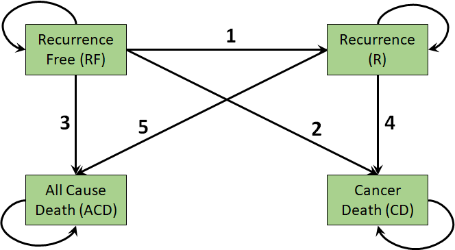
Our application is the Colon cancer dataset previously explored in the context of cohort Markov models in Chapter 9.(Moertel et al., 1995; Moertel et al., 1990) The 4-state multistate model is illustrated in Figure 11.1. In this case there are \(H=4\) health states so the \(Q\) matrix from Section 11.1 is a \(4 \times 4\) matrix. The 4 permitted transition rates make up the off-diagonal elements of this matrix.
The permitted transitions in continuous time are numbered, labelled, and described below.
| Transition number | Abbreviation | Description |
|---|---|---|
| 1 | RF to R | Recurrence-Free to Recurrence |
| 2 | RF to OCD | Recurrence-Free to Dead (Other cause) |
| 3 | R to CD | Recurrence to Dead (Cancer) |
| 4 | R to OCD | Recurrence to Dead (Other cause) |
This model is irreversible as individuals cannot return to their previous states (e.g., no transitions from recurrence to recurrence-free). Note again that these are different from the permitted transitions over an interval of time. For example, over one year, an individual can transition from recurrence-free to cancer death, but in a continuous-time model we assume that this happened via a transition to recurrence at some point in the year.
Each state will be associated with an annualised cost and utility which will be used to estimate total costs and QALYs as in Section 11.1.5.
There are again 3 strategies under investigation:
- Observation (Obs), i.e., no treatment
- Levamisole (Lev)
- Levamisole and fluorouracil (Lev+5FU)
These strategies are assumed to affect only the transition from recurrence-free to recurrence (RF to R). Other than this, they are also associated with a cost and risk of toxicity. Toxicities themselves have an impact on costs and QALYs. These are further specified below as we develop code for the model.
11.3 Case study: Colon data
Unlike in the Markov model chapter where transitions between states were represented by probabilities, we will now be fitting survival models to the time-to-event data in the underlying dataset. The basic data are stored in msm_colon and are loaded and displayed below.
load(file = "data/msm_colon.rda")
dim(msm_colon)
[1] 3663 11# Add numeric strategy that will be used in survival and multistate modelling
msm_colon$strategy_id <- as.numeric(msm_colon$rx)
# Look at the contents
head(msm_colon) id rx age sex from to Tstart Tstop years status trans strategy_id
1 1 Lev+5FU 43 1 1 2 0.00000 2.650240 2.650240 1 1 3
2 1 Lev+5FU 43 1 1 3 0.00000 2.650240 2.650240 0 2 3
3 1 Lev+5FU 43 1 1 4 0.00000 2.650240 2.650240 0 3 3
4 1 Lev+5FU 43 1 2 3 2.65024 4.164271 1.514031 1 4 3
5 1 Lev+5FU 43 1 2 4 2.65024 4.164271 1.514031 0 5 3
6 2 Lev+5FU 63 1 1 2 0.00000 8.451745 8.451745 0 1 3# Give a description of the transition numbers in msm_colon
transition_names <- c("RF to R", "RF to OCD", "R to CD", "R to OCD")There are 3663 rows which include observed times of transition between states, and censored times of transitions to “competing risks” - transitions that a person was at risk of, but didn’t happen. For example, the first person in this dataset transitioned from state 1 to state 2 at 2.65 years (first row). This transition event implies a censoring time of 2.65 for the “competing” transition from state 1 to state 4 (second row).
The names of the 4 transitions are stored in transition_names. The id is the individual identifier while rx specifies their treatment. The rx codes are 1 for Obs, 2 for Lev, and 3 for Lev+5FU.
Columns age and sex are self-explanatory while from and to are the starting and finishing state of each transition. Tstart gives the time that individual started in the from state while Tstop gives the time they exit that state and move to to. The year column gives the time spent in state from. Finally, status indicates if the transition was actually observed (1) or if it was censored (0). For example, a transition from RF to R would be censored if the individual moved to OCD before they had a recurrence. The final column trans specifies the transition number, as per the above table.
11.4 Estimating multistate models using fully-observed data
Given the colon dataset in the required format, we can fit the time-to-event models to inform our clock-reset 4-state colon cancer model. We first load the necessary packages survival and flexsurv and set a random seed.
library(survival)
library(flexsurv)
set.seed(2549788)
We then choose a set of distributions to explore for each transition, and assign names to the latter. For illustration, we will consider only the common parametric survival models, but fractional polynomials, Royston-Parmar splines, and piecewise-exponential models are other common choices and supported by hesim.
distribution_names <- c(
  "exp", "weibull", "gompertz", "lognormal", "llogis", "gamma"
)
transition_names <- c("RF to R", "RF to OCD", "R to CD", "R to OCD")
For simplicity of presentation, we will choose the model with minimum Akaike Information Criterion (AIC) on the observed data for each transition (Burnham and Anderson, 2002). However, we will be using the survival models for extrapolation so in practice they should be compared to long-term data, rather than selected by minimum AIC (Jackson et al., 2016; Latimer, 2013). That approach would be better aligned with guidance from institutions such as NICE and further detail is given in Chapter 7.
To implement minimum AIC selection, we will build the table survival_aic_cr to compare the performance of distributions for transitions in our clock-reset model. Note that we can choose different distributions for each transition.
# Matrix to store summaries of the clock-reset distributions
survival_aic_cr <-
  matrix(nrow = length(distribution_names),
         ncol = length(transition_names),
         dimnames = list(distribution_names, transition_names))

# Lists to store actual survival models for use in multistate models
survival_models_cr <- list()
We will use the flexsurvreg() function from flexsurv() and Surv from survival to fit these survival models to the msm_colon dataframe. The treatments are assumed to only affect transitions from recurrence-free to recurrence (RF to R). We further assume no other covariate effects on transition rates. We specify the models in a list survival_formula_cr. Applying the Surv() function to the Tstart and Tstop columns of msm_colon would use time since entering the model (or dataset) as the time parameter of the survival models, and would thus result in a clock-forward model. We will instead apply Surv() to years so as to use the time spent in the current state as the time variable, and thus obtain clock-reset models for each transition.
# List of distributions fit to time-in-state (years column of msm_colon)
survival_formula_cr <- list()
# Set the transitions that depend on treatment
survival_formula_cr[["RF to R"]] <- as.formula(
  "Surv(years, status) ~ factor(strategy_id)"
)
# Set the transitions that are independent of treatment
survival_formula_cr[["RF to OCD"]] <- as.formula("Surv(years, status) ~ 1")
survival_formula_cr[["R to CD"]] <- as.formula("Surv(years, status) ~ 1")
survival_formula_cr[["R to OCD"]] <- as.formula("Surv(years, status) ~ 1")
We loop over transitions i_trans and distributions i_dist fitting the models and extracting the AIC. The subset = (trans == i_trans) argument specifies that only transitions i_trans should be used, while dist specifies the distribution. The output survival model object of flexsurvreg() includes an AIC element which we can extract. The code for the loop is below.
for(i_trans in 1:length(transition_names)) {
  survival_models_cr[[transition_names[i_trans]]] <- list()
  for(i_dist in 1:length(distribution_names)) {
    # Fit the survival distribution for this transition
    survival_models_cr[[i_trans]][[distribution_names[i_dist]]] <-
      flexsurvreg(survival_formula_cr[[i_trans]],
                  subset = (trans == i_trans),
                  data = msm_colon, dist = distribution_names[i_dist])

    # Save the AIC for model comparison
    survival_aic_cr[i_dist, i_trans] <-
      survival_models_cr[[i_trans]][[distribution_names[i_dist]]]$AIC
  }
}
For each of the transitions in our model we can now choose the distribution with minimum AIC. The min_aic_table is set up below to store the AIC and selected distribution.
# Which models have the lowest AIC?
min_aic_table <- matrix(NA, nrow = 2, ncol = length(transition_names))
rownames(min_aic_table) <- c("CR distribution", "CR AIC")
colnames(min_aic_table) <- transition_names
min_aic_table["CR distribution", ] <- distribution_names[
  apply(survival_aic_cr, c(2), which.min)
]
min_aic_table["CR AIC", ] <- round(
  apply(survival_aic_cr, c(2), min), digits = 2
)
Looking at the results, we can see that the selection is a Gompertz or exponential for all transitions, with the only exception being a log-logistic for recurrence (R) to cancer death (CD). Given these selections, we could proceed to build a multistate model.
| RF to R | RF to OCD | R to CD | R to OCD | |
|---|---|---|---|---|
| CR distribution | gompertz | exp | gompertz | llogis |
| CR AIC | 2535.87 | 403.48 | 3211.49 | 1202.3 |
11.5 Using msm to estimate multistate models using panel data
In this section we show how to use the msm package to estimate constant transition rates if we have only panel observed data. To do this, msm uses the likelihood described in Section 11.1.3. If fully-observed, or complete case, data are available, the more flexible methods of Section 11.4 should be used.
We first load the (artificial) panel observed version of the colon data and view its contents. This is a series of observations of the state occupancy for each individual id on strategy_id at timepoint years. These were generated by simulating 10 random observation times for each individual and checking their state occupancies at those times. The times of death are taken to represent the exact time of death, but with the state of disease unknown at the instant before death.
We can use msm::statetable.msm() to summarise the number of observed transitions between states in successive observations. For example, we see that there were 383 transitions from recurrence-free to recurrence and 2 transitions from recurrence to all-cause death. This could alert us that estimates of the transition rate from recurrence to dead other-cause may not be reliable. There are zero transitions from recurrence to recurrence-free, as the model in Figure 11.1 is assumed to be irreversible.
Note that this table describes the transitions over an interval. We do not actually know the times of all transitions that happened in continuous time. For example, 41 people appeared to “transition” from the “Recurrence-free” state to the “Dead (Cancer)” state over some interval of time. However, these people must have experienced recurrence of cancer in this interval, even though the “Recurrence” state was not directly observed.
# Load the msm library
library(msm)
load("data/panel_colon_data.rda")
# Look at the contents
head(panel_colon)
id strategy_id age sex years state
2 1 3 43 1 1.063052 1
3 1 3 43 1 2.183803 1
4 1 3 43 1 2.209600 1
5 1 3 43 1 2.487186 1
6 1 3 43 1 3.790750 2
7 1 3 43 1 3.818891 2# Summarise the transitions
statetable.msm(state, id, data = panel_colon) to
from 1 2 3 4
1 4023 383 41 466
2 0 1211 367 2To fit a multistate model to this panel data, first we need to specify the allowed transitions in continuous time. Here, these are stored in a \(4 \times 4\) matrix colon_qmatrix, which is passed as the qmatrix argument to msm. The entry in row \(r\) and column \(s\) is 1 if an instantaneous transition in continuous time is allowed from state \(r\) to state \(s\). Here the four transitions represent recurrence, death from cancer given recurrence, and death from other causes from either of the living states. As we noted, the transition from “Recurrence-free” to “Dead (Cancer)” is not allowed.
The first argument of the msm::msm() function indicates the name of the state variable and the time variable in the data. The covariates argument indicates the explanatory variables. As explained in Section 11.2, treatment strategies are assumed to affect only the transition from recurrence-free to recurrence (RF to R). We have therefore specified the strategy_id to be a predictor only of recurrence (the \(1 \rightarrow 2\) transition), and not of death from cancer (the \(2 \rightarrow 3\) transition) or death from other causes (\(1 \rightarrow 4\) and \(2 \rightarrow 4\)).
The data are taken to be intermittent observations by default, but an exception here is for the two death states (states 3 and 4), where we suppose we know the time of entry exactly, but not the disease state at the instant before death. This observation scheme is indicated here by the deathexact argument.
The final argument to msm() is center = FALSE which ensures the intercepts represent covariate values of zero, easing interpretation. Using center = TRUE would align the intercepts with the mean covariates.
colon_qmatrix <- rbind(
  c(0, 1, 0, 1),
  c(0, 0, 1, 1),
  c(0, 0, 0, 0),
  c(0, 0, 0, 0)
)

rownames(colon_qmatrix) <- colnames(colon_qmatrix) <-
  c("Recurrence-free", "Recurrence", "Dead (Cancer)", "Dead (Other cause)")

# Estimate the transition rates
colon_msm_fit <- msm(state ~ years, subject = id, data = panel_colon,
                    covariates = list (
                      "1-2" = ~ strategy_id
                    ),
                    deathexact = c(3, 4),
                    qmatrix = colon_qmatrix,
                    gen.inits = TRUE,
                    center = FALSE)
The resulting object colon_msm_fit can be visualised by calling it on the R workspace.
Call:
msm(formula = state ~ years, subject = id, data = panel_colon,
qmatrix = colon_qmatrix, gen.inits = TRUE, covariates = list(`1-2` = ~strategy_id),
deathexact = c(3, 4), center = FALSE)

Maximum likelihood estimates
Baselines are with covariates set to 0

Transition intensities with hazard ratios for each covariate
                                     Baseline
Recurrence-free - Recurrence-free    -0.094329 (-0.103690,-0.08581)
Recurrence-free - Recurrence          0.050239 ( 0.042752, 0.05904)
Recurrence-free - Dead (Other cause)  0.044090 ( 0.040085, 0.04850)
Recurrence - Recurrence              -0.385315 (-0.424537,-0.34972)
Recurrence - Dead (Cancer)            0.375742 ( 0.340013, 0.41523)
Recurrence - Dead (Other cause)       0.009573 ( 0.002458, 0.03728)
                                     strategy_id2         strategy_id3
Recurrence-free - Recurrence-free
Recurrence-free - Recurrence         1.034 (0.8272,1.292) 0.5519 (0.433,0.7036)
Recurrence-free - Dead (Other cause) 1.000                1.0000
Recurrence - Recurrence
Recurrence - Dead (Cancer)           1.000                1.0000
Recurrence - Dead (Other cause)      1.000                1.0000

-2 * log-likelihood:  9515.441
Note that with intermittently-observed data such as this, care is needed to ensure that all of the parameters can be estimated from the data. It is common for intermittently-observed data to not contain any information about one of the transition intensities or covariate effects. In such a case, the msm function will either return an error message, or produce estimates with implausibly large confidence intervals. This can be tested in advance by tabulating and exploring the data, as we did with statetable.msm(). This could have happened if we had placed a covariate effect on all transition intensities. If a treatment effect had been included on the \(2 \rightarrow 4\) transition, for example, the sparsity of the data would have lead to extreme confidence intervals for this effect.
Examining data summaries (e.g. statetable.msm) can help to identify where data are weak, but many problems can be avoided by excluding implausible parameters based on background knowledge. Here we might expect that treatment does not affect the risk of non-cancer death, and direct transitions from recurrence-free to death from cancer are not possible.
By fitting the model, the transition intensities and covariate effects are estimated. We can convert these to transition probabilities using the msm::pmatrix.msm() function. For models that have covariates, we should also indicate for which covariate categories to estimate the transition probabilities. As an example, here we estimate for the first strategy. We see that roughly 4% of recurrence-free individuals are expected to have experienced recurrence and still be alive within a year. Also, of those individuals having a recurrence, about 31% are expected to have cancer related death within a year.
pmatrix.msm(colon_msm_fit, covariates = list(strategy_id = 1)) Recurrence-free Recurrence Dead (Cancer) Dead (Other cause)
Recurrence-free 0.9099833 0.03966592 0.00807061 0.042280140
Recurrence 0.0000000 0.68023659 0.31181935 0.007944065
Dead (Cancer) 0.0000000 0.00000000 1.00000000 0.000000000
Dead (Other cause) 0.0000000 0.00000000 0.00000000 1.000000000We will later use these panel data estimates to simulate costs and QALYs with hesim.
11.6 Cost-effectiveness modelling with multistate models in hesim
We will use the hesim package package to implement individual-level continuous-time clock-reset multistate models for colon cancer. We begin with the fully-observed case of Section 11.4 before returning to the panel estimates of Section 11.5.
As explained in Chapter 9 we use probabilistic analyses, where uncertainty in the input parameters is propagated to the estimated costs and effects, as our base case. This is due to deterministic analyses being biased by the non-linearity of the total costs and effects functions (Thom et al., 2022; Wilson, 2021). We thus name it probabilistic analysis rather than probabilistic sensitivity analysis (PSA). As noted in Chapter 9, this approach is supported by organisations such as NICE and CADTH (CADTH, 2023; NICE, 2022).
11.6.1 Setting up hesim and specifying the model
We first load the necessary packages (including flexsurv again) and specify variables that define the model. The package data.table provides the data table structure used by hesim. This is the colon multistate model already described but we now set the number of probabilistic samples (n_samples) and number of simulated individuals (n_patients) each to 1000. We use “patients” rather than “individuals” for consistency with hesim internal variable names.
# data.table package provides the data structures for hesim
library(data.table)
library(flexsurv)
library(hesim)
library(ggplot2)
library(BCEA)

# Global variables that specify the model
state_names <- c(
  "Recurrence-free", "Recurrence", "Dead (Cancer)", "Dead (Other cause)"
)
treatment_names <- c("Observation", "Lev", "Lev+5FU")
n_patients <- 1000
n_samples <- 1000
n_states <- 4
n_treatments <- 3
The four permitted transitions now need to be assigned a unique consecutive number in the transition_matrix that links them to the relevant states. Transitions that are not permitted (e.g., recovering from R to RF), and the diagonal entries, are set to NA.
# Four transitions: 1 (RF to R), 2 (RF to OCD), 3 (R to CD), 4 (R to OCD)
transition_matrix <- rbind(
  c(NA, 1, NA, 2),
  c(NA, NA, 3, 4),
  c(NA, NA, NA, NA),
  c(NA, NA, NA, NA)
)
colnames(transition_matrix) <- rownames(transition_matrix) <- state_names
The strategies are also given unique consecutive numbers strategy_id in the strategies data table below. This table also includes the string strategy_name for readability. The patients for simulation are also a data table with consecutive numeric patient_id but also with selected baseline characteristics. The only characteristics defined in this case are age and sex. Baseline risk or other disease characteristics could be included.
An idiosyncrasy of hesim is that the states data table only needs to give numeric and string names for the non-absorbing states (i.e., R and RF but not CD or OCD).
# Treatments to compare
strategies <- data.table(
  strategy_id = c(1, 2, 3),
  strategy_name = treatment_names
)

# Individuals are randomly sampled with replacement from the colon dataset
# Sample patient IDs to preserve correlation between age and sex
patient_id_sample <- sample(1:n_patients, size = n_patients, replace = TRUE)
patients <- data.table(
  patient_id = 1:n_patients,
  age = msm_colon$age[patient_id_sample],
  sex = msm_colon$sex[patient_id_sample]
)

# Only need to specify the non-death (i.e., non-absorbing) states as hesim adds
# death/absorbing states automatically based on the transition matrix
states <- data.table(
  state_id = c(1:2),
  state_name = rownames(transition_matrix)[1:2]
)
There are several utility functions in hesim that make the inputs and outputs more readable. The hesim_data() function is used to create lists of strategies, patients, and states for simulation, while expand() duplicates patients for each strategy. The get_labels() function lets users create nice labels for treatment strategies, subgroups, health states, and/or transitions when presenting results.
# hesim data specification
hesim_data_ <- hesim_data(
  strategies = strategies,
  patients = patients,
  states = states
)

# Duplicate the individual data for each treatment strategy
transition_model_data <- expand(hesim_data_,
  by = c("strategies", "patients")
)


# Use hesim to generate model labels
hesim_labels <- get_labels(hesim_data_)
hesim_labels$transition_id <- c(
  "RF to R" = 1,
  "RF to OCD" = 2,
  "R to CD" = 3,
  "R to OCD" = 4
)

hesim_labels$state_id <- c(1:n_states)
names(hesim_labels$state_id) <- state_names
11.6.2 Building the disease simulation model in hesim
The disease simulation is constructed using survival models on each of the transitions. The models for each transition are stored as lists of flexsurvreg objects created by the flexsurvreg_list() function. These selections are as described in Section 11.4.
# List of survival models for each transition
hesim_survival_cr <- flexsurvreg_list(
  survival_models_cr[["RF to R"]][["gompertz"]],
  survival_models_cr[["RF to OCD"]][["gompertz"]],
  survival_models_cr[["R to CD"]][["llogis"]],
  survival_models_cr[["R to OCD"]][["exp"]]
)
The most important function when setting up a hesim individual-level continuous-time transition model is the create_IndivCtstmTrans() function, which creates an object of class IndivCtstmTrans. All objects in hesim are implemented using the R6 package, which provides object oriented programming functionality for R. The create_IndivCtstmTrans() function takes as its arguments the lists of flexsurvreg objects, the individual-level transition model data output by expand(), the trans_mat transition matrix, and n the number of samples. The final argument is clock and this can be "reset", "forward", or "mix", with the latter allowing some transitions to be clock-reset and others clock-forward.
# Calling the constructor for IndivCtstmTrans
transition_model_cr <- create_IndivCtstmTrans(
  hesim_survival_cr, transition_model_data,
  trans_mat = transition_matrix,
  n = n_samples,
  clock = "reset",
  start_age = patients$age
)
11.6.3 Building the utility models in hesim
In hesim the utility and cost models are specified as unique values for all combinations of strategy, state, individual, sample, and time. We start with the utilities but costs are a similar process. In the colon cancer model these are a combination of the state utility and disutility due to treatment toxicity, both of which are randomly sampled. There are two time periods as well. In the first year individuals have a risk of toxicity and associated disutility, and thereafter they only experience state utility. We therefore need unique values for each state, sample, and treatment, and for each of the two time periods. A blank utility_table with this flexibility is constructed using the hesim function stateval_tbl() below.
# Two time periods for utilities
n_utility_times <- 2

# We sample these utilities and probabilities separately and combine into a
# table of "custom" utilities for hesim
# Number of states is the number of states minus the number of absorbing states
# which is 2 in this case.

utility_table <- stateval_tbl(
  data.table(
    strategy_id = rep(
      # Table defines values for each treatment
      c(1:n_treatments),
      each = length(states$state_id) * n_utility_times * n_samples
      ),
    sample = rep(
      # Table then gives values for each sample
      rep(c(1:n_samples),
        each = length(states$state_id) * n_utility_times
        ),
      # Sample values repeated for each treatment
      times = n_treatments
      ),
    state_id = rep(
      # Values for each state
      rep(1:length(states$state_id),
        each = n_utility_times
        ),
      # State values repeated for each treatment and state
      times = n_treatments * n_samples
      ),
    time_start = rep(
      # Values for each timepoint
      c(0, 1),
      # Timepoint values repeated for each treatment, sample, and state.
      times = n_treatments * n_samples * length(states$state_id)
      ),
    value = 1
  ),
  dist = "custom"
)

head(utility_table)
sample strategy_id state_id time_id time_start time_stop value
<int> <int> <int> <int> <num> <num> <num>
1: 1 1 1 1 0 1 1
2: 1 1 1 2 1 Inf 1
3: 1 1 2 1 0 1 1
4: 1 1 2 2 1 Inf 1
5: 2 1 1 1 0 1 1
6: 2 1 1 2 1 Inf 1The uncertainty about state utilities is specified with a Normal distribution, as are the probabilities and disutilities of toxicity for each treatment.
# Normally distributed state utilities
utility_recurrence_free <- rnorm(n_samples, 0.8, sd = 0.1 * 0.8)
utility_recurrence <- rnorm(n_samples, 0.6, sd = 0.1 * 0.6)

# Probability and disutility of toxicity
# No SD reported so use 10% of the mean
p_tox_lev <- rnorm(n_samples, mean = 0.20, sd = 0.1 * 0.20)
p_tox_lev5fu <- rnorm(n_samples, mean = 0.40, sd = 0.1 * 0.40)
disutility_toxicity <- rnorm(n_samples, mean = -0.1, sd = 0.1 * 0.1)
Given the blank utility_table and samples for utilities, probabilities of toxicity, and disutilities of toxicity, we can calculate the combined utilities. For example, the utility for Lev individuals in the recurrence-free state (state_id == 1) in the first year is calculated as utility_recurrence_free + p_tox_lev * disutility_toxicity and in later years is utility_recurrence_free.
# Fill in the blank utility table

# Utilities for Observation
# Not affected by disutility and the same for first and subsequent years
utility_table[strategy_id == 1 & state_id == 1, "value"] <-
  c(
    utility_recurrence_free,
    utility_recurrence_free
  )
utility_table[strategy_id == 1 & state_id == 2, "value"] <-
  c(
    utility_recurrence,
    utility_recurrence
  )

# Utilities for Lev
utility_table[strategy_id == 2 & state_id == 1, "value"] <-
  c(
    utility_recurrence_free + p_tox_lev * disutility_toxicity,
    utility_recurrence_free
  )
utility_table[strategy_id == 2 & state_id == 2, "value"] <-
  c(
    utility_recurrence + p_tox_lev * disutility_toxicity,
    utility_recurrence
  )

# Utilities for Lev+5FU
utility_table[strategy_id == 3 & state_id == 1, "value"] <-
  c(
    utility_recurrence_free + p_tox_lev5fu * disutility_toxicity,
    utility_recurrence_free
  )
utility_table[strategy_id == 3 & state_id == 2, "value"] <-
  c(
    utility_recurrence + p_tox_lev5fu * disutility_toxicity,
    utility_recurrence
  )
The filled in utility_table, hesim_data_ model specification, and number of samples are then passed to the hesim::create_StateVals(). This creates the utility_model object, which is a stateval_tbl object specifying utilities for, in the colon cancer case, each state, sample, treatment, and the two time periods.
utility_model <- create_StateVals(utility_table,
  hesim_data = hesim_data_,
  n = n_samples
)
11.6.4 Building the cost models in hesim
The cost models are specified in a very similar way to the utility models, except that there are now two models. One is for treatment or Drug costs and the other is for state costs which hesim names the ongoing Medical costs. In our example, treatment costs are applied once at the start of the model and there is a unique value for each treatment and sample. State costs are zero except for a one-off cost of $40,000 for advanced treatment in the recurrence state.
# Treatment costs depend on the costs of adverse events which are a one-off
treatment_cost_table <- stateval_tbl(
  data.table(
    strategy_id = rep(c(1:n_treatments), each = n_samples),
    sample = rep(c(1:n_samples), times = n_treatments),
    value = 1
  ),
  dist = "custom"
)

# State costs are zero except for one-off cost of advanced treatment
# in recurrence state
n_cost_times <- 2

state_cost_table <- stateval_tbl(
  data.table(
    state_id = rep(states$state_id, each = n_cost_times),
    time_start = rep(c(0, 1), times = length(states$state_id)),
    est = c(0, 0, 40000, 0)
  ),
  dist = "fixed"
)
We then define the distribution for the toxicity cost and combine it with the treatment cost and probabilities of toxicity to calculate treatment costs.
# Normally distributed cost of toxicity
cost_toxicity <- rnorm(n_samples, mean = 2000, sd = 0.1 * 2000)


treatment_cost_table[strategy_id == 1, "value"] <- 0
treatment_cost_table[strategy_id == 2, "value"] <- 5000 +
  p_tox_lev * cost_toxicity
treatment_cost_table[strategy_id == 3, "value"] <- 10000 +
  p_tox_lev5fu * cost_toxicity
Finally, we pass our treatment_cost_table and state_cost_table to create_StateVals() to create the treatment and state cost models. These are stored in the cost_models list with elements for Drug and Medical costs.
treatment_cost_model <- create_StateVals(treatment_cost_table,
  n = n_samples,
  hesim_data = hesim_data_
)
state_cost_model <- create_StateVals(state_cost_table,
  n = n_samples,
  hesim_data = hesim_data_
)
cost_models <- list(Drug = treatment_cost_model,
  Medical = state_cost_model
)
11.6.5 Simulating from the combined cost-effectiveness model
Simulation of the disease progression, costs, and utilities is done in hesim by creating an R6 object of type IndivCtstm (Individual-level continuous-time state-transition model, where state-transition is a synonym for multistate). The constructor function IndivCtstm$new() takes as arguments the IndivCtstmTrans objects we created in Section 11.6.2, the StateVals object utility_model from Section 11.6.3, and the StateVals object cost_models from Section 11.6.4.
# Build the combined economic models of progression, costs, and utilities
economic_model_cr <- IndivCtstm$new(
  trans_model = transition_model_cr,
  utility_model = utility_model,
  cost_models = cost_models
)
Simulation is conducted by calling functions of the IndivCtstm objects. The sim_disease() function simulates disease and creates the public member object disprog_, meaning disease progression, which is a form of data table. The columns of disprog store the transitions from a state entered at time_start to another state at time_stop. These are simulated for each sample, strategy_id, and patient_id. The grp_id relates to subgroups but we are not analysing subgroups in this application so all are set to 1.
# Disease modelling
economic_model_cr$sim_disease()

head(economic_model_cr$disprog_)
sample strategy_id patient_id grp_id from to final time_start time_stop
<num> <int> <int> <int> <num> <num> <int> <num> <num>
1: 1 1 1 1 1 4 1 0.0000000 14.2074939
2: 1 1 2 1 1 2 0 0.0000000 0.8518056
3: 1 1 2 1 2 4 1 0.8518056 3.8322418
4: 1 1 3 1 1 2 0 0.0000000 1.3263604
5: 1 1 3 1 2 4 1 1.3263604 1.7410480
6: 1 1 4 1 1 4 1 0.0000000 14.1280744With the disease progression in disprog_ the functions sim_costs() and sim_qalys() can be used to simulate discounted costs and QALYs, respectively, with a single argument dr specifying the discount rate. We use the 3% rate common in the US setting (Haacker et al., 2020).
# Simulate discounted costs and qalys using the simulated disease progression
economic_model_cr$sim_costs(dr = 0.03)
economic_model_cr$sim_qalys(dr = 0.03)
State occupancy probabilities can also be calculated from disprog_ using the sim_stateprobs() function. This takes a vector of timepoints t at which the probabilities should be estimated.
# State occupancy probabilities for clock-reset
economic_model_cr$sim_stateprobs(t = seq(0, 20 , 1/12))
The results of these state probability calculations are stored in state_probs_. In the code below we use the autoplot() function, which is from the ggplot2 package but adapted for hesim objects. This averages probabilities within strategies, labels with treatment and state names, and then plots over time.
state_probabilities_cr <- economic_model_cr$stateprobs_[
  , .(prob_mean = mean(prob)),by = c("strategy_id", "state_id", "t")
]

autoplot(economic_model_cr$stateprobs_, labels = hesim_labels)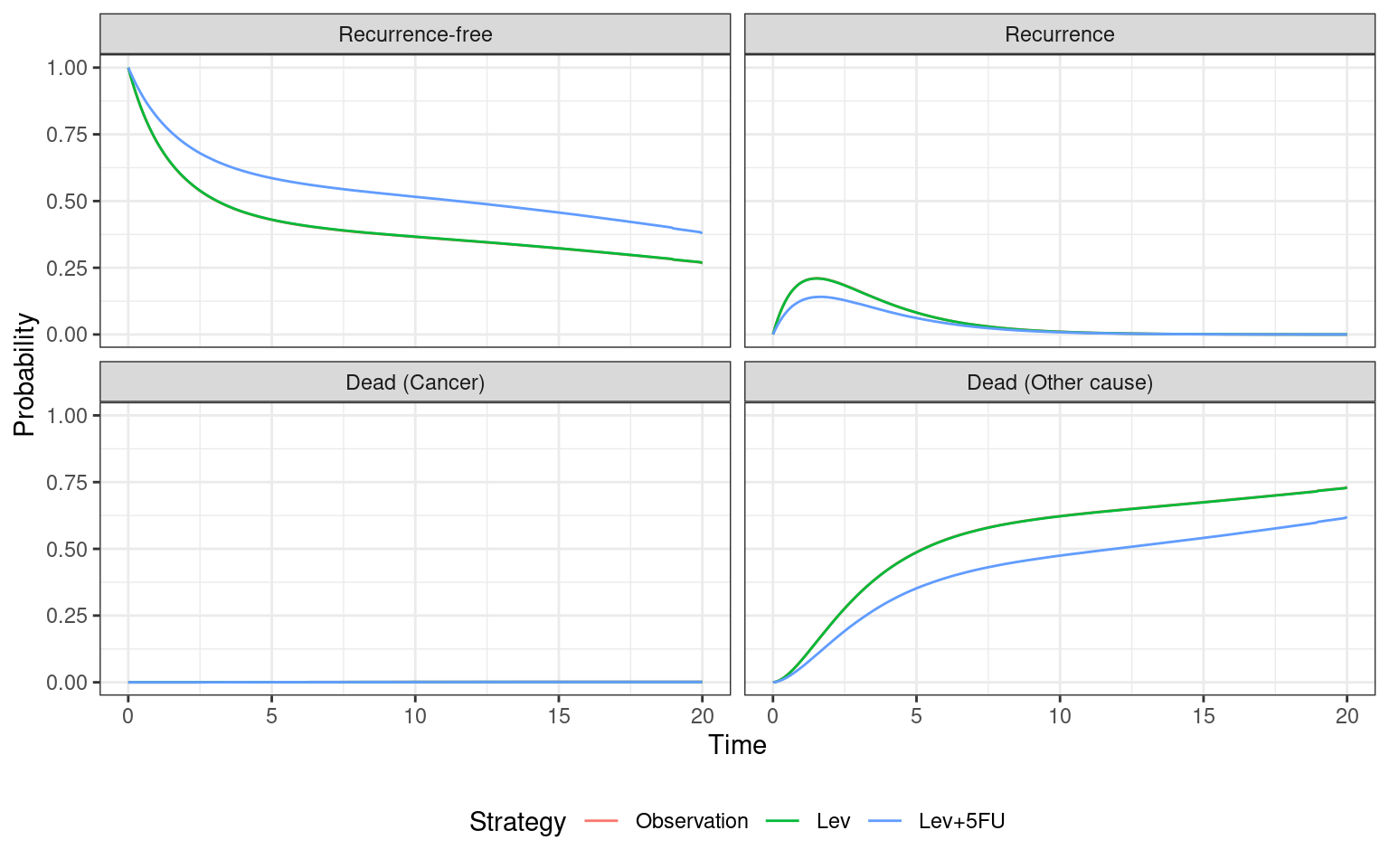
11.6.6 Analysing the results using hesim and BCEA
We analyse the results using the package BCEA, which provides various functions to summarise samples or simulations of total costs and effects. We first need to convert the output from hesim into the format expected by BCEA. The BCEA package requires matrices of costs and effects, each with a row each for probabilistic samples and a column for each treatment. The code below uses the summarize() function of the IndivCtstm object economic_model_cr to calculate total costs and QALYs over the simulated time horizon and averaged over all individuals.
# Generate matrices suitable for use by BCEA
hesim_summary_cr <- economic_model_cr$summarize()
We then reformat this output into the costs_matrix_dr and effects_matrix_dr matrices.
# Convert costs and QALYs into a matrix usable by BCEA
# n_samples rows and n_strategies columns
costs_matrix_cr <- effects_matrix_cr <-
  matrix(NA,
  nrow = n_samples,
  ncol = n_treatments,
  dimnames = list(NULL, treatment_names)
)


for(i_treat in 1:n_treatments) {
  costs_matrix_cr[, i_treat] <- with(
    hesim_summary_cr$costs,
    costs[category =="total" &
      strategy_id == i_treat &
      dr == 0.03]
  )

  effects_matrix_cr[, i_treat] <- with(
    hesim_summary_cr$qalys,
    qalys[strategy_id == i_treat &
    dr == 0.03]
  )

}
The final step is to pass these to the BCEA::bcea() function, specifying ref=1 so that Observation is the reference treatment. Net benefits are calculated up to a maximum willingness-to-pay threshold of Kmax=200000. This gives the colon_bcea_cr object which can be used for cost-effectiveness analysis using BCEA.
# Generate and return the BCEA object
colon_bcea_cr <- bcea(
  eff = effects_matrix_cr,
  cost = costs_matrix_cr,
  ref = 1,
  interventions = treatment_names,
  Kmax = 200000
)
A quick check of the means and 95% credible intervals for costs and effects can be conducted using apply and standard statistical functions. This shows that Lev has higher costs and lower effects than Observation, and is thus dominated. This is aligned with the discrete-time cohort Markov models of Chapter 9. Lev+5FU has substantially higher costs than Observation but also has substantially higher effects.
# Quick check of costs and effects
apply(
  costs_matrix_cr, 2, function(x) {
    c(mean(x), quantile(x, probs = c(0.025, 0.975)))
  }
)
Observation Lev Lev+5FU
4899.400 52214.99 123716.74
2.5% 4009.278 40446.30 90935.47
97.5% 5920.848 63381.89 153400.23apply(
effects_matrix_cr, 2, function(x) {
c(mean(x), quantile(x, probs = c(0.025, 0.975)))
}
) Observation Lev Lev+5FU
6.805412 6.726762 8.551542
2.5% 4.868503 4.661727 5.783697
97.5% 9.302382 8.983880 11.788233The first function from BCEA to apply is summary with a willingness-to-pay threshold of wtp equal to $100,000/QALY. These results show that Lev has lower net benefit than Observation but that Lev+5FU has greater net benefit than both Lev and Observation. The ICER for Lev+F5U is below the $100,000/QALY willingness-to-pay commonly used in US markets (Menzel, 2021; Pichon-Riviere et al., 2023).
# CE Analysis using clock-reset model
summary(colon_bcea_cr, wtp = 100000)
Cost-effectiveness analysis summary

Reference intervention:  Observation
Comparator intervention(s): Lev
                          : Lev+5FU

Optimal decision: choose Observation for k < 68400 and Lev+5FU for k >= 68400


Analysis for willingness to pay parameter k = 1e+05

            Expected net benefit
Observation               675642
Lev                       620461
Lev+5FU                   731438

                          EIB  CEAC    ICER
Observation vs Lev      55181 0.862 -601597
Observation vs Lev+5FU -55796 0.179   68046

Optimal intervention (max expected net benefit) for k = 1e+05: Lev+5FU

EVPI 5531.3
The BCEA::ceplane.plot() function is used below to plot the cost-effectiveness plane. The limits of the costs and effects axes have been manually selected to give the most representative plot. This illustrates that Lev+5FU clearly has higher costs and, as most points are in the positive range of the x-axis, most likely has higher effects than Observation. The majority of the points are below the willingness-to-pay threshold of $100,000/QALY.
# Change object so that comparisons are against Lev+5FU
# Generate and return the BCEA object
colon_bcea_lev5fu_cr <- bcea(
  eff = effects_matrix_cr,
  cost = costs_matrix_cr,
  ref = 3,
  interventions = treatment_names,
  Kmax = 200000
)

# Plot the cost-effectiveness plane for Lev+5FU vs Observation
ceplane.plot(colon_bcea_lev5fu_cr,
  wtp = 100000,
  comparison = 1,
  xlim = c(-2, 4),
  ylim = c(-20000, 160000),
  graph = "ggplot2"
) +
  ylab("Incremental costs ($)")  +
  xlab("Incremental effects (QALYs)")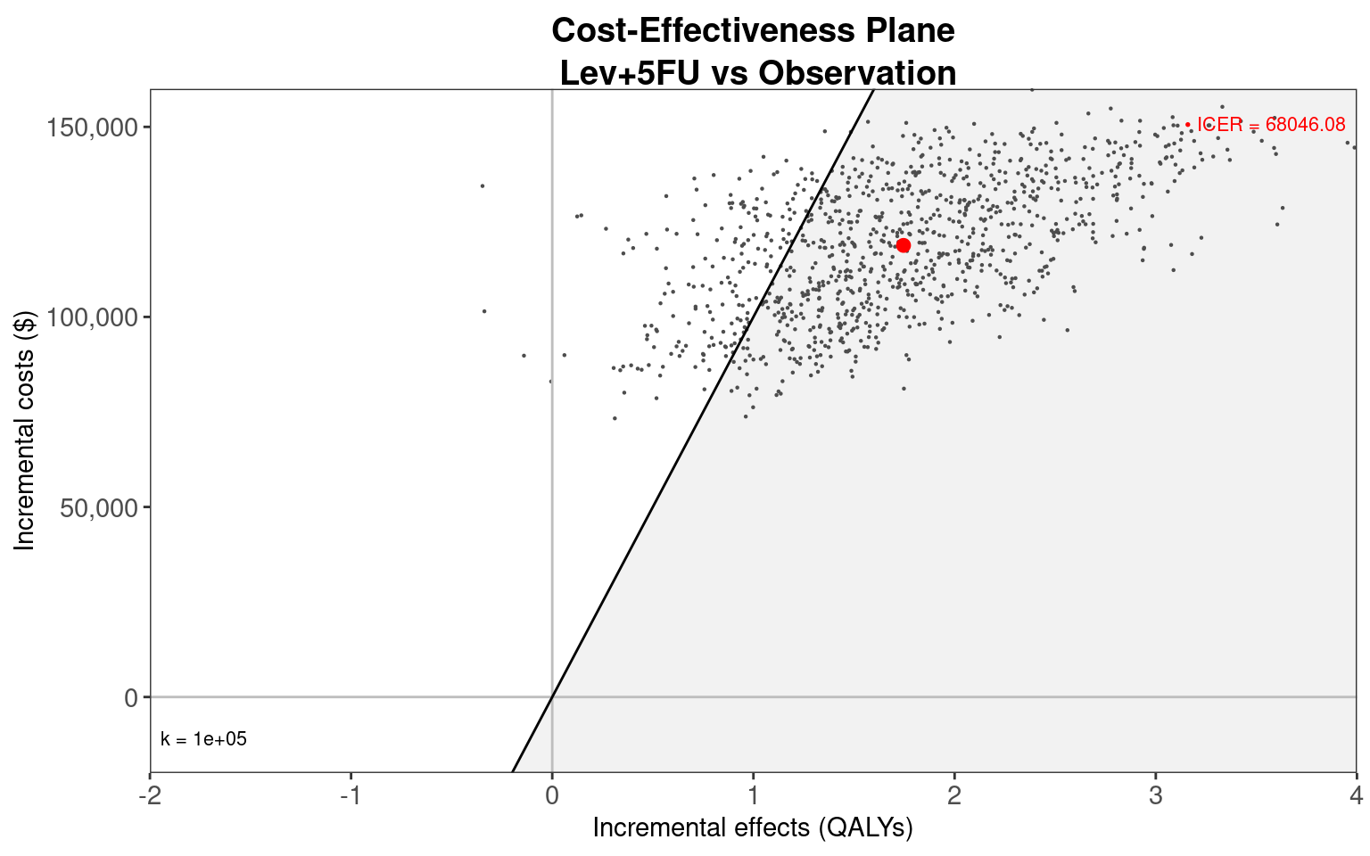
The final plot is a cost-effectiveness acceptability curve, generated using the BCEA::multi.ce() and BCEA::ceac.plot() functions. There is uncertainty up to $70,000/QALY about which of Observation or Lev+5FU is most cost-effective. However, in the $100,000/QALY to $150,000/QALY range Lev+5FU has a probability of 60-90% of having the highest net benefit. Lev+5FU would therefore be recommended.
# Plot a CEAC
colon_multi_cr <- multi.ce(colon_bcea_cr)
ceac.plot(colon_multi_cr,
  graph = "ggplot",
  line = list(color = c("red", "green", "blue")),
  pos = c(0, 0.50)
) +
  xlab("Willingness-to-pay ($)")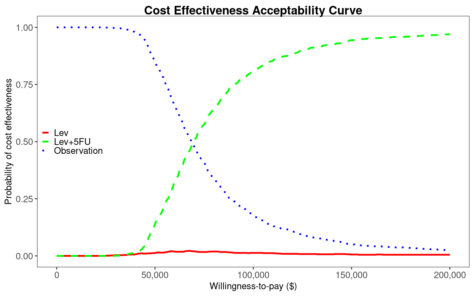
11.6.7 Cost-effectiveness modelling using estimates from panel data
We now repeat the analysis using the colon_msm_fit object of constant (log) hazard rates estimated by msm in Section 11.5. The estimates of the log hazard rates and log hazard ratios are stored in the colon_msm_fit$estimates vector and the covariance matrix in colon_msm_fit$covmat matrix. The elements of this vector and matrix are arranged so that the intercept terms are first given for each transition (i.e., the log hazard rates for Observation), then the log hazard ratios for the first covariate (i.e., treated with Lev), and then the log hazard ratios for the next covariate (i.e., treated with Lev+5FU). In the code below we sample from the multivariate Normal distribution for log hazard rates and give the elements of these samples meaningful names.
# Sample from the multivariate Normal for log hazard rates estimated by msm
# using panel data
transition_parameter_names <- paste(
  rep(c("RF to R", "RF to OCD", "R to CD", "R to OCD"), 3),
  rep(c("Intercept", "Lev", "Lev+5FU"), each = 4)
)

panel_parameter_samples <- MASS::mvrnorm(
  n = n_samples,mu = colon_msm_fit$estimates,Sigma = colon_msm_fit$covmat
)
colnames(panel_parameter_samples) <- transition_parameter_names
panel_parameter_samples <- as.data.frame(panel_parameter_samples)

for (i in paste("RF to CD", c("Intercept", "Lev", "Lev+5FU")))
  panel_parameter_samples[[i]] <- 0
The hesim package can interact with the output of msm but only if fitting a discrete-time cohort model using the hesim::create_CohortDtstmTrans() function. However, we can manually provide the panel_parameter_samples above as samples for the individual-level continuous-time model through a hesim::params_surv_list list, each of which is a hesim::params_surv object. These objects can be any parametric or flexibly parametric survival model, but the outputs of msm are simple exponential distributions. They require only the appropriate intercept and coefficients for each treatment. These are extracted from panel_parameter_samples below.
# Transition model parameters based on msm panel data
transition_model_parameters <- params_surv_list(
  # Distribution for first transition "RF to R"
  params_surv(
    coefs = list(data.frame(
      intercept = panel_parameter_samples[, "RF to R Intercept"],
      "Lev" = panel_parameter_samples[, "RF to R Lev"],
      "Lev+5FU" = panel_parameter_samples[, "RF to R Lev+5FU"])
    ),
    dist = "exp"),
  # Distribution for second transition "RF to OCD"
  params_surv(
    coefs = list(data.frame(
      intercept = panel_parameter_samples[, "RF to OCD Intercept"],
      "Lev" = panel_parameter_samples[, "RF to OCD Lev"],
      "Lev+5FU" = panel_parameter_samples[, "RF to OCD Lev+5FU"])
    ),
    dist = "exp"),
  # Distribution for third transition "R to CD"
  params_surv(
    coefs = list(data.frame(
      intercept = panel_parameter_samples[, "R to CD Intercept"],
      "Lev" = panel_parameter_samples[, "R to CD Lev"],
      "Lev+5FU" = panel_parameter_samples[, "R to CD Lev+5FU"])
    ),
    dist = "exp"),
  # Distribution for fourth transition "R to OCD"
  params_surv(
    coefs = list(data.frame(
      intercept = panel_parameter_samples[, "R to OCD Intercept"],
      "Lev" = panel_parameter_samples[, "R to OCD Lev"],
      "Lev+5FU" = panel_parameter_samples[, "R to OCD Lev+5FU"])
    ),
    dist = "exp")
)
Once we have our params_surv_list object transition_model_parameters we can pass it to hesim::create_IndivCtstmTrans() to generate the requisite transition model. Since msm assumes the multistate model is clock-forward, we need to specify the clock = "forward" argument, rather than setting it to clock-reset. We also need to ensure that the input_data argument matches the covariates specified in transition_model_parameters. To do this, we add an intercept covariate which is always 1 and covariates for treatment with Lev and Lev+5FU that match the naming in transition_model_parameters.
# Need to have data matching the terms of transition_model_parameters
transition_model_data$"intercept" <- 1
transition_model_data$"Lev" <- transition_model_data$strategy_name == "Lev"
transition_model_data$"Lev.5FU" <-
  transition_model_data$strategy_name == "Lev+5FU"

# msm fit using factor for strategy but hesim data for strategy is numeric
transition_model_data$strategy_id <-
  as.numeric(transition_model_data$strategy_id)

# Use the panel data transition models
transition_model_panel <- create_IndivCtstmTrans(transition_model_parameters,
  input_data = transition_model_data,
  trans_mat = transition_matrix,
  clock = "forward",
  start_age = patients$age
)
Simulation using this clock-forward model uses the same code as for the clock-reset model.
# Combine with the same cost and utility models used for the clock-reset model
economic_model_panel  <- IndivCtstm$new(
  trans_model = transition_model_panel,
  utility_model = utility_model,
  cost_models = cost_models
)

# Simulate disease, costs, effects, and state probabilities
economic_model_panel$sim_disease()
economic_model_panel$sim_costs(dr = 0.03)
economic_model_panel$sim_qalys(dr = 0.03)
economic_model_panel$sim_stateprobs(t = seq(0, 20 , 1/12))
Given the differences between models (i.e., fully-observed vs panel data, non-constant hazards vs exponential, clock-reset vs clock-forward) it is interesting to first compare the estimated state probabilities. We see that differences between treatments are much less pronounced, due to the more limited data and lack of flexibility in the exponential survival models. However, Lev+5FU individuals spend marginally more time in the recurrence-free state and have a slightly lower rate of cancer death.
# Explore state probabilities
state_probabilities_panel <- economic_model_panel$stateprobs_[
  , .(prob_mean = mean(prob)),by = c("strategy_id", "state_id", "t")
]

autoplot(economic_model_panel$stateprobs_, labels = hesim_labels)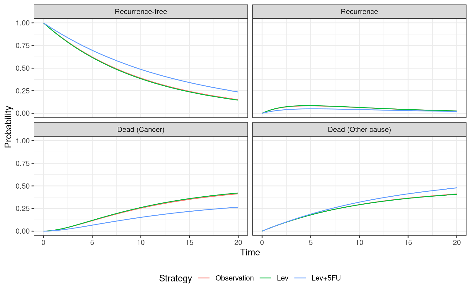
hesim_summary_panel <- economic_model_panel$summarize()

# Convert costs and QALYs into a matrix usable by BCEA
# n_samples rows and n_strategies columns
costs_matrix_panel <- effects_matrix_panel <-
  matrix(NA, nrow = n_samples, ncol = n_treatments,
         dimnames = list(NULL, treatment_names))


for(i_treat in 1:n_treatments) {
  costs_matrix_panel[, i_treat] <- with(
    hesim_summary_panel$costs,
    costs[category =="total" &
    strategy_id == i_treat &
    dr == 0.03]
  )

  effects_matrix_panel[, i_treat] <- with(
    hesim_summary_panel$qalys,
    qalys[strategy_id == i_treat &
    dr == 0.03]
  )

}

# Quick check of costs and effects
apply(
  costs_matrix_cr, 2, function(x) {
    c(mean(x), quantile(x, probs = c(0.025, 0.975)))
  }
)
Observation Lev Lev+5FU
4899.400 52214.99 123716.74
2.5% 4009.278 40446.30 90935.47
97.5% 5920.848 63381.89 153400.23apply(
effects_matrix_cr, 2, function(x) {
c(mean(x), quantile(x, probs = c(0.025, 0.975)))
}
) Observation Lev Lev+5FU
6.805412 6.726762 8.551542
2.5% 4.868503 4.661727 5.783697
97.5% 9.302382 8.983880 11.788233In the $50,000/QALY to $100,000/QALY range, Lev+5FU is again the most cost-effective intervention and it has the highest expected net benefit at $100,000/QALY.
Lev is again dominated, with higher costs and lower effects than Observation. We can extract total costs and QALYs and pass these to BCEA for processing. We see that there is greater uncertainty between Observation and Lev+5FU in the $100,000/QALY to $150,000/QALY range, with both interventions having 25-75% probability of being most cost-effective in this region. This greater uncertainty reflects the use of partially observed data. The Markov assumption and use of constant transition rates, rather than time-varying rates of the clock-reset model, are also potentially biasing results. We would recommend using the clock-reset model with flexible survival distributions for decision making.
# Generate and return the BCEA object
colon_bcea_panel <- bcea(
  eff = effects_matrix_panel,
  cost = costs_matrix_panel,
  ref = 1,
  interventions = treatment_names,
  Kmax = 200000
)

# CE Analysis using panel data model
summary(colon_bcea_panel, wtp = 100000)
Cost-effectiveness analysis summary

Reference intervention:  Observation
Comparator intervention(s): Lev
                          : Lev+5FU

Optimal decision: choose Observation for k < 124000 and Lev+5FU for k >= 124000


Analysis for willingness to pay parameter k = 1e+05

            Expected net benefit
Observation               687695
Lev                       624092
Lev+5FU                   666731

                         EIB  CEAC    ICER
Observation vs Lev     63604 0.980 -294624
Observation vs Lev+5FU 20964 0.722  123714

Optimal intervention (max expected net benefit) for k = 1e+05: Observation

EVPI 7335.5
# Plot a CEAC
colon_multi_panel <- multi.ce(colon_bcea_panel)
ceac.plot(colon_multi_panel,
graph = "ggplot",
line = list(color = c("red", "green", "blue")),
pos = c(0, 0.50)
) +
xlab("Willingness-to-pay ($)")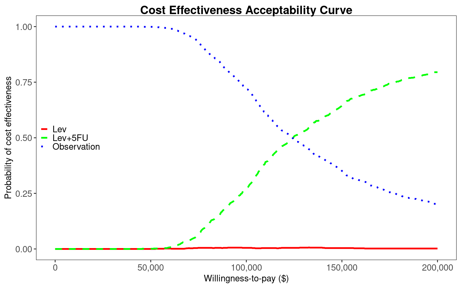
11.7 Discussion
In this chapter we have explored more general multistate modelling, building on the discrete-time cohort Markov models described in Chapter 9. Generalisations included a switch from discrete-time to continuous-time, from cohort to individual-level simulation, and relaxations of the Markov assumption. In Section 11.1 we discussed the concepts of transition intensity rates and how their dependence on time through time-in-model or time-in-state lead to clock-forward or clock-reset models, respectively. These concepts were illustrated in Section 11.2 through the colon cancer case study from Chapter 9. Using this case study, we explained the estimation of transition rates using both fully-observed data using flexsurv in Section 11.4 and panel data using msm in Section 11.5. We presented a general hesim implementation of multistate models for cost-effectiveness analysis in Section 11.6. This included the use of the data.table package for specifying utility models in Section 11.6.3 and cost models in Section 11.6.4. This specification of the structure was common to both clock-reset and clock-forward models, but specifics of their simulations were provided in Section 11.6.5 and Section 11.6.7, respectively. Finally, we explained the use of BCEA to analyse the total costs and effects estimated by our hesim colon cancer models.
We have attempted to keep our implementations as general as possible. The code for the 4-state clock-reset and clock-forward models could be adapted to other oncology settings. This would require replacing the msm_colon data on for time to progression, cancer death, and other death and rerunning the flexsurv survival modelling, or rerunning the msm rate estimation on a replacement panel data for panel_colon. With the underlying multistate model replaced, it would then be necessary to update the strategy names, and cost data specified by treatment_cost_table and state_cost_table, and the utility data specified in utility_table. The structure of the multistate model could be changed by first changing n_states and transition_matrix. Our application only included baseline data on age and sex. Our transition rate models did not include dependence on these covariates. This could be modified to better model individual heterogeneity by simply including age or sex, or other regressions on other covariates (the "Surv(years, status) ~ " expressions passed to flexsurvreg() and covariates in msm()) and then passing these generalised models to hesim.
Despite the data and modelling differences, we came to similar conclusion about the optimal treatments between the clock-reset fit to fully-observed data, clock-forward fit to panel data, and the discrete-time cohort Markov model in Chapter 9. Lev was dominated by Observation under all models. Lev+5FU had greater effects and costs than Observation and thus became more cost-effective with greater willingness-to-pay. We found uncertainty to be greater when using panel data, and the greater flexibility of the clock-reset model fit to fully-observed data makes it our recommended option for decision making. However, this only applies when fully-observed data on all relevant outcomes and strategies are available, which is rarely the case.
Our colon cancer application assumed that only one dataset was needed (or available) to inform event times on our strategies of interest. In practice, it is likely that indirect treatment comparison (ITC) using multiple studies would be required (Hoaglin et al., 2011; Jansen et al., 2011). The most common for of ITC is network meta-analysis (NMA), which was described in Chapter 10. The hesim package can use estimated log hazard ratios from a proportional hazards NMA and the coefficients of standard parametric, fractional polynomial, or spline models from non-proportional hazards NMA (Cope et al., 2023; Freeman et al., 2022; Woods et al., 2010). Instead of passing a flexsurvreg_list object to create_IndivCtstmTrans() it is possible to instead pass params_surv_list of params_surv objects. One params_surv object must be provided for each possible transition. These take a dist argument for the distribution (e.g., "gompertz" for a Gompertz, "fracpoly" for fractional polynomials, or "survspline" for splines), a coef argument for samples of the coefficients, and a distribution-specific aux argument. This allows great flexibility in the form of the NMA or ITC that can be input to hesim. This includes population adjusted hazard ratios from matching adjusted indirect comparison (MAIC) or multilevel network meta-regression (ML-NMR) (Phillippo et al., 2020, 2018).
In the oncology space, if only published Kaplan-Meier (KM) curves on Overall Survival (OS) and Progression Free Survival (PFS) are available for some comparators, a partitioned survival model may be more appropriate (Woods et al., 2017). This avoids the necessity of assuming that rates of pre-death progression are the same as rates of progression or death (i.e., PFS), which is often assumed for multistate models fit to OS and PFS KM curves (Jansen et al., 2023; Woods et al., 2020). Partitioned survival models are explained in Chapter 7 but can also be implemented in hesim. The major disadvantage of partitioned survival models is that OS and PFS are assumed to be independent, which is not necessarily true and can lead to extrapolated OS being greater than PFS (Woods et al., 2020). Methods have been developed that can separate pre-progression and post-progression death by identifying ties in the OS and PFS data, thus allowing estimates of the transition rates necessary for multistate models (Pahuta et al., 2019). A recent method allows the simultaneous conduct of NMA and multistate model estimation and maintains the structural link between OS and PFS (Jansen et al., 2023). These methods further reduce the justification for using partitioned survival models rather than multistate models.
We have presented only one way of implementing clock-reset and clock-forward multistate models. An important alternative is the mstate package (Wreede et al., 2011). This allows for both estimation of clock-forward and clock-reset models but also the simulation necessary for cost-effectiveness modelling (Williams et al., 2017). Our multistate models were not fully general as individual history is only included through their current state and their current time-in-state (i.e., semi-Markov models). For example, the time to transition from recurrence-free to recurrence is not used by the model after the transition occurs, so rates of cancer death do not depend on this initial transition time. The hesim package does not currently allow for such history to be stored so a base R implementation would be required (Krijkamp et al., 2018). The method of discrete event simulation (DES) allows for full history to be used but at the cost of greater computational requirements. Such models are described in detail in Chapter 12.
In summary, we have provided generalisable R code for estimating and simulating from individual-level continuous-time multistate models under the clock-reset and clock-forward assumptions. The colon cancer example can be adapted to other oncology datasets. The multistate model can be extended to other state structures, to use other survival models, and to incorporate ITCs. Partitioned survival models provide an alternative approach when only OS and PFS KM curves are available, but recent methods have now allowed the direct estimation of rates needed for multistate models. Full individual history can be used through implementation in base R or through use of DES. On the latter, we refer the interested reader to Chapter 12.