7 Introduction to survival analysis in HTA

Christopher Jackson
MRC Biostatistics Unit, University of Cambridge, Cambridge, UK

Nick Latimer
University of Sheffield, UK

Jeroen Jansen
University of California, San Francisco, USA

Petros Pechlivanoglou
The Hospital for Sick Children and University of Toronto, Toronto Canada

Gianluca Baio
University College London, UK

7.1 Introduction: Survival Analysis in Health Economics

In this chapter we demonstrate how to undertake survival analysis in the context of economic evaluation and decision modeling. This area is vast, and involves many complex issues. We cannot cover everything, but aim to outline the most important issues, providing advice and guidance on how to implement relevant survival analysis techniques in R for the purpose of informing an economic evaluation. Whilst we refer to “survival” analysis, we are actually referring to “time-to-event” analysis, where the event of interest could be anything that can happen after some time — it may be disease progression, treatment failure, or death.

7.1.1 Aims of Economic Evaluation

Economic evaluations are typically conducted to inform resource allocation decisions. Healthcare budgets are limited and funds need to be allocated in a way that maximise benefits. The extent to which this is explicitly done varies across health systems, and the way benefits are measured also differs. But, the fact remains that economic evaluation and health technology assessment are undertaken to compare competing interventions to inform decision making. Decisions are made around what treatments should be available in the health system and are mostly made at the population level. For decisions to be sound, it is crucial for all relevant comparators to be analysed, and for the relevant costs and benefits (which may differ depending upon the perspective taken in the analysis) to be accurately estimated and included. For interventions that affect survival, accurately estimating expected survival for each comparator is of paramount importance, and it is equally important that complete survival distributions are estimated. Treatments are given to entire disease populations, not just median patients. If distributions are skewed, that must be taken into account by using an appropriate survival distribution to estimate mean survival for each competing intervention.

7.1.2 Evidence used to inform survival estimates

New drugs are usually licensed by regulators on the basis of evidence from randomised controlled trials (RCTs). RCTs represent the gold-standard of evidence, with randomisation providing assurance that at the beginning of the trial known and unknown confounders (characteristics that are associated with both treatment and the outcome) will be balanced between randomised treatment groups. Whilst RCTs represent an excellent source of evidence on the effectiveness of interventions, they are limited in two ways that are particularly relevant for this chapter.

7.1.3 RCTs are limited in duration

Clinical trials do not continue forever. Usually a proportion of patients will not have experienced the event of interest at the end of the trial. Those who remain free of the event at the end of trial follow-up are censored at that point. The survival function, which describes the probability of survival (i.e. not experiencing the event of interest) over time — often estimated using the Kaplan-Meier estimator — does not reach zero. Therefore, estimates of mean survival that are restricted to the duration of the trial will be underestimates of the true mean. For this reason, to arrive at survival estimates that are relevant for economic evaluation, we must extrapolate beyond the observed survival data. This is typically done using parametric models. Parametric survival models assume that the time-to-event data follow a certain parametric distribution. Therefore, in this chapter we do not focus on non parametric models such as the Kaplan-Meier estimator or semi-parametric models such as the Cox proportional hazards model in any detail. Whilst both are common survival analysis techniques, neither are parametric, and therefore they cannot be used for extrapolation. Instead we focus on parametric models, of which there are many, each making different assumptions about hazard functions (the instantaneous risk of the event occurring in small intervals through time). These assumptions determine the shape of survival curves and can result in drastically diverging estimates of mean survival. Attempting to identify appropriate models with which to extrapolate survival, and to adequately characterise uncertainty around these, represents a fundamental part in economic evaluations of interventions that affect survival.

7.1.4 RCTs rarely include all relevant comparators

Usually RCTs compare a new intervention to placebo, best supportive care, or one carefully selected alternative. This is problematic when, as is often the case, it is important for resource allocation decisions to compare the intervention in question to other treatments, against which it has not been compared in an RCT. Network meta-analysis forms the basis of a chapter in this book (see Chapter 4 for a more detailed description), but there are important factors that must be considered specific to a survival analysis context which are addressed in this chapter.

7.1.5 Structure of the chapter

In Section 7.2 we provide an overview of standard parametric models and their specification. We show how these can be fit to survival or time-to-event data and demonstrate approaches for choosing between models. For simplicity, we consider a case where patient-level data are available from an RCT and we demonstrate fitting a survival model to a single arm of the trial. In reality, patient-level data are often not available to researchers. For this reason we provide a section on how to create pseudo patient-level data by digitising published summary data. Model choice should be based upon a consideration of fit to the observed data, but also on the validity of model extrapolations. To judge this, information external to the RCT is likely to be required. Research is ongoing in this area, but Sections 7.2 and 7.4.3 provide advice.

Section 7.3.1 considers the estimation of treatment effects. Whilst Section 7.2 demonstrates fitting survival models for one treatment, in reality we will need to (at least) fit survival models that predict survival for two or more arms of an RCT. This requires assumptions about the nature of the treatment effect.

In Section 7.4 we move beyond standard parametric survival distributions. We introduce and demonstrate more complex models, such as flexible (spline-based) parametric models, mixture models and cure models.

In Section 7.5 we move beyond the simple case where only the interventions included in a single RCT need to be compared, providing an outline and illustration of network meta-analysis in a survival setting.

Section 7.6 and Section 7.7 run through a worked example and describe the all important process of reconstructing survival data from published graphical summaries, such as Kaplan-Meier curves (which we introduce in Section 7.2).

Finally, in Section 7.8 we discuss how to incorporate outputs from survival analyses into economic models. We consider economic models that are structured as partitioned survival models and as state transition models, and provide advice on incorporating uncertainty.

Throughout the chapter we will be using the colon cancer example dataset colon, which is provided within the survival R package to guide the implementation of the various concepts in an R setting

7.2 Parametric modelling of a single survival distribution

7.2.1 Survivor and hazard functions

Suppose we wish to estimate the distribution of survival times from data giving observed survival times for a set of patients. Firstly we will formalise the problem with some notation and definitions. The survival time is the time from some starting event of interest \(t=0\) until the patient’s death (or time to some other event of interest). In a randomised trial, for example, \(t=0\) would represent the time of randomisation. Then let \(T\) denote the random variable that governs a patient’s survival time. A defining characteristic of survival times is that they are non-negative. We want to estimate the distribution of \(T\). The distribution can be expressed in various forms. Two particularly useful ways to do this for survival analysis are:

the survivor function (often referred to as the survival function) \(S(t) = P(T > t)\): this represents the chance of surviving up to a certain time \(t\). A defining characteristic of survival times is that they are non-negative.The survivor function is related to the cumulative distribution function \(F(t) = 1 - S(t) = \Pr(T \leq t)\), but is often more common and practical to focus on survival probability.
The hazard function \(h(t)\), which can be written in different ways: \[ \begin{aligned} h(t) &= \lim_{\delta t \rightarrow 0} \frac{\Pr(T < t + \delta t \mid T > t)}{\delta t}\\ &= \lim_{\delta t \rightarrow 0} \frac{S(t) - S(t + \delta t)}{\delta t S(t)}\\ & = \frac{f(t)}{S(t)} \end{aligned} \] where \(f(t)\) is the probability density function.

The hazard at time \(t\) describes the instantaneous risk of death for someone who is still alive at this time. The value of the hazard is less easily understood than the value of the survivor function, because the hazard is not a probability, but a rate, so can be greater than 1. However, when considered as a function of time, the hazard gives an intuitive idea of how the risk of death for a person currently alive, or the force of mortality, changes through time. This interpretation will be used throughout the chapter when choosing, assessing and comparing models.

Important

In fact, we recommend that the hazard function is thoroughly explored in applied work to gain insights into the underlying assumptions of, and inference obtained from, a specific parametric model. For instance, exploring the hazard function can highlight inconsistencies in the model extrapolation (e.g. instantaneous risks of death that are too small at a very advanced age).

In general, suppose we have a sample of data giving observed times for \(n\) individuals \(t_i: i=1,\ldots, n\). Some of the \(t_i\) represent observed times of death or event of interest. The rest of the \(t_i\) represent times of censoring, which means that the person was observed to be still alive or not having experienced the event of interest at \(t_i\), but their eventual time-to-event is unknown. Let \(d_i=1\) if \(t_i\) be an observed death time, or \(d_i=0\) if \(t_i\) be a time of censoring. These data are collectively denoted \((\boldsymbol{t},\boldsymbol{d})\).

Right Censoring

Right censoring is a defining feature of time-to-event data and occurs because, for various reasons, we may not be able to observe the occurrence of a particular outcome, which we know will eventually happen (e.g. death). Thus, the absence of the observation cannot be taken at face value, because we know that sooner or later the event will happen. For this reason, it is crucial to account for right censoring in the modelling of survival data.

Censoring could also be considered as a form of missing data mechanism (see Chapter 6), in the sense that we do not have complete information on some individuals. Some common situations are as follows.

Commonly in trials and other medical studies, everyone is followed up until a specified date. Therefore for those who are still alive, their time of death / event of interest is known only to be after this date, hence is right-censored. This situation is known as administrative censoring. An advantage of this kind of data is that censoring is non-informative, or censoring happens at random, which means that the time that someone will be censored (being chosen in advance, by design of the study) is unrelated to the time when they will die/ experience the event.
In other situations, individuals may drop out before the planned end of the study, again giving right-censored data. The assumption of censoring at random may be unrealistic, if the fact that an individual has dropped out of the “risk set” (i.e. the set of individuals at risk of experiencing the event) is influenced by the individual’s circumstances and characteristics. If those characteristics are also predictors of their eventual death time, then ignoring this extra information will result in biased estimates of the survival distribution. However there are some methods available to account for informative censoring (Grafféo et al., 2019).
Left censoring may sometimes occur in clinical studies, for example, when the time at which the event of interest occurs is known precisely, but the time at which the individual enters the risk set is not.
Interval censoring occurs if the event of interest is only known to have happened within two dates or time points, but the precise time is not known.

More generally, a censored observation of a random variable is one whose value is not known exactly, but only known to be within some range. In this book chapter we will only deal with right censored data, that is, event times known only to be greater than some value. More general forms of censoring are supported in the packages that we use, however. Likewise we do not deal with truncated data, which describes situations where individuals are only observed if they have survived for (or died before) a particular length of time.

There are numerous estimators available to for the survival function \(S(t)\). The most common is the Kaplan-Meier non-parametric estimator. Assuming \(d_i\) is the number of events observed at time interval \(t_i\) and \(n_i\) the number of individuals at risk at time \(t_i\), the Kaplan-Meier estimate can be defined as

\[ \begin{aligned} \widehat{S(t)} &= \prod_{t_i \leq t }\frac{n_i - d_i}{n_i} \end{aligned} \]

7.2.2 The Colon Cancer example

The main example used to illustrate this chapter is taken from an RCT that was performed in the 1980’s to investigate the efficacy of post-surgery adjuvant therapy for colon cancer (Moertel et al., 1995). It can be accessed using the colon command in the survival R package . The trial included three arms: i) Observation (Obs), ii) Levamisole (Lev), iii) Levamisole and fluorouracil (Lev+5FU). The outcome of interest is recurrence of cancer or death. Figure 7.1 shows Kaplan-Meier estimates \(\widehat{S_r(t)}\) of the recurrence-free survival probability \(S_r(t)\) as a function of treatment group \(r\) and time since randomisation. The estimate is produced with the survfit function from the survival package, and plotted using ggsurvplot from the survminer package (Kassambara et al., 2021) . Survival is greatest in the Levanisole+5-FU arm, and most of the deaths in the data have occurred by 5 years. Around half the population is alive without their cancer having recurred by 5 years, and the time to death or recurrence for these people is right-censored at points ranging from 5 to 10 years.

# extract RFS and CSS data
# the dataset is structured so that each row represents a possible outcome.
# the variable etype defines if the outcome is recurrence (etype = 1) or death
# (etype = 2). We first create the composite outcome of recurrence or death in 
# order to create a recurrence free survival outcome. 

colon_all <- inner_join(x = subset(colon, etype ==1),
                        y = subset(colon[,c("id","time","status","etype")],
                                   etype ==2),
                        by = "id",suffix=c("RFS","OS"))
colon_all[colon_all$statusOS == 1                 &
          colon_all$timeOS   <= colon_all$timeRFS,"statusRFS"] = 1  

colon_all      <- colon_all %>% mutate(yearsRFS = timeRFS / 365.25)
colon_all      <- colon_all %>% mutate(yearsOS  = timeOS / 365.25)

RFS_data   <- colon_all %>% dplyr::select(id, rx, statusRFS, yearsRFS)%>%
                            mutate(years = yearsRFS, status = statusRFS)
RFS_lev    <- RFS_data %>% dplyr::filter(rx=="Lev")
RFS_obs    <- RFS_data %>% dplyr::filter(rx=="Obs")
RFS_lev5fu <- RFS_data %>% dplyr::filter(rx=="Lev+5FU")
KM_RFS     <- survfit(Surv(time = years, event = status) ~ rx, data = RFS_data)

# plot KM for RFS
pal <- c("gray8", "gray87", "gray56")
ggsurvplot(
  KM_RFS,
  data = RFS_data,
  size = 1,                  # change line size
  palette = pal,             # custom color palettes
  conf.int = FALSE,          # Add confidence interval
  pval = FALSE,              # Add p-value
  risk.table = TRUE,         # Add risk table
  risk.table.height = 0.25,  # Useful to change when you have multiple groups
  ggtheme = theme_bw(),      # Change ggplot2 theme
  xlab     = 'Years since randomisation',     # Change X-axis label
  title    = "Survival curve for Recurrence Free Survival",
  subtitle = "Based on Kaplan-Meier estimates"
)

Figure 7.1: Kaplan-Meier estimates for the recurrence-free survival probability, as a function of the treatment group

Figure 7.2 shows estimates of the hazard \(h(t)\) as a function of time for each treatment group. These are computed by kernel density estimation, a nonparametric method, using the muhaz package (Hess and Gentleman, 2021), and with 95% confidence intervals obtained by bootstrapping. For the chemotherapy groups we see a peak in the hazard after one year, and in all groups there is a decrease over time up to at least 5 years. While the point estimates of the hazard suggest an increase after 5 years for the Levamisole group, this is based on a small amount of data (17 people at risk in this group after 7.5 years) and the confidence intervals also include the possibility of a decrease.

Figure 7.2: Estimates for the hazard function in each treatment group

7.2.3 Fitting parametric survival models to data

In this section we show how to fit parametric survival models to time-to-event data. This involves defining a specific form for \(S(t \mid \boldsymbol{\theta})\) or, equivalently, for the hazard \(h(t\mid\boldsymbol{\theta})\), so that the survival probability at time \(t\) can be defined as a function of \(t\) and a small number of parameters (collectively termed \(\boldsymbol{\theta}\)) that characterise the distribution. Some examples are given in the next section. Then the likelihood of this model (see Section 4.4.2), given the data above, is comprised of two products with the first product representing the joint probability of the data for people \(i\) whose death times were observed at \(t_i\), and the second representing the joint probability of the data for people who were censored at \(t_i\). For now, we are supposing that all people have the same survival distribution. In Section 7.4 we will relax this assumption.

In a frequentist framework, the parameters \(\boldsymbol{\theta}\) can be estimated by maximising the likelihood as a function of \(\boldsymbol{\theta}\) (see Section 4.4.2). Just as importantly, as well as providing a point estimate for the parameters, we should also characterise our uncertainty about this estimate, given the evidence (Section 1.7.1).

7.2.4 Estimating mean survival and extrapolation

In health economic evaluations, the choice of intervention can have consequences for lifetime survival. Therefore we often want to estimate the expected survival over a long, or even lifetime, horizon, \[ \mbox{E}[T \mid \boldsymbol{\theta}]= \int_0^\infty S(t)dt. \tag{7.1}\]

Equation 7.1 implies that the expected (i.e. mean) survival time can be computed as the “area under the survival curve”. More importantly, this clarifies why applications of survival modelling in HTA require a full extrapolation of the survival curve: the focus of the economic analysis is on the mean survival time and in order to obtain it, we need to be able to derive the full survival curve in the range of times \(t=0,\ldots,\infty\).

A challenge with estimating lifetime survival based on trial data is that we can only observe death times \(T\) that are shorter or equal to the follow-up time of the trial. For people still alive at the end of the trial, the survival times are right-censored. To estimate \(E(T)\), we need to know the distribution of \(T\) over all plausible values of \(T\).

This can be estimated by using a parametric model, under an important assumption. We must assume that the functional form \(h(t\mid\boldsymbol{\theta})\) chosen for the hazard, and the parameters \(\boldsymbol{\theta}\) that this depends on, are the same for all \(T\), both before and after the maximum follow-up time \(t^*\) of the data. For example, suppose the trial data give evidence that the hazard is constant up to the maximum follow up time \(t^*\) of the study. We can infer that the expected survival is \(\displaystyle\mbox{E}(T) = \int_0^\infty S(t\mid\boldsymbol{\theta})dt\) if we assume that the hazard also remains constant for future times \(t>t^{*}\), at the value inferred from the short term data. This is why this procedure is commonly referred to as extrapolating survival data: information gained from shorter term data is assumed to apply over the longer term. Careful judgement is required to assess whether the assumption is reasonable, which depends on the extent of censoring (thus how much of the distribution of \(T\) can be identified from the data) and knowledge of the disease and treatment.

Note that as long as half of the population have died (or experienced the event of interest) by \(t^*\), the median survival can be estimated, e.g. from a Kaplan-Meier curve, without any extrapolation. For example, in the colon cancer example (Figure 7.1), the median survival in the Levamisole group is 2.8 years, the time \(t\) when \(S(t)=0.5\). However, as discussed in Chapter 1, the expected outcome is more relevant when the decision-maker aims to maximise the overall benefits for a population.

In some situations, the follow up of the trial is long enough to capture meaningful differences in survival between the health policies being compared. In these cases, a useful quantity to estimate is the restricted mean survival time \(\int_{0}^{t^{*}} S(t) dt\) (Royston and Parmar, 2013), the expected time up to \(t^*\) years spent alive, which would only require extrapolation if \(t^*\) is beyond the follow up of the trial.

7.2.5 Examples of survival models

In parametric survival modelling, parametric forms can be assumed for the survival or the hazard function which are thought to represent many plausible ways that the risk of death could vary through time. This can often be done by appropriately defining the hazard function. In a few situations, the hazard might be constant through time. The Exponential distribution has \(S(t) = \exp(-\lambda t)\), and a constant hazard \(h(t)=\lambda\). However, in many situations, we would want to allow the hazard to depend on time \(t\). One commonly-used distribution that allows hazard to be time-dependent is the Weibull distribution, whose hazard form is \(h(t)=\lambda t^\alpha\), which is increasing for \(\alpha>1\), decreasing for \(\alpha<1\) or constant through time for \(\alpha=1\).

More generally, a wide range of parametric forms are available in standard R packages. A selection of the most commonly used ones, and their distinctive characteristics, are are described briefly in Table below. Among other packages, these can all be fitted in the R package flexsurv (Jackson, 2016) which includes an extensive vignette with worked examples. Awkwardly, some of these distributions have different parameterisations or definitions in different software or literature, but the definitions used in this book are those used in flexsurv. Formulae for the survival functions, and details of how to fit the corresponding models in R, are given in the vignettes in the flexsurv package (Jackson, 2016).

Distribution	Characteristics of the hazard function
Exponential	Constant hazard \(\lambda\)
Weibull	Increasing, decreasing or constant hazard with time \(\lambda t^\alpha\)
Gamma	Increasing, decreasing or constant hazard with time (complex mathematical form)
Gompertz	Exponentially-increasing hazard \(\lambda\exp(\alpha t)\) with time, which has been used to model human survival at older ages
Log-normal	Unimodal hazard, i.e. increasing to a maximum before decreasing to zero (complex mathematical form)
Log-logistic	Decreasing hazard, or similar to the log-normal
Generalized gamma	Includes the gamma, Weibull and log normal as special cases (in the formulation of Prentice, 1975).

However, we do not recommend simply fitting every model that is available, without thoughtful consideration of what hazard shape each model implies. This is particularly important if we need to extrapolate beyond the data in order to estimate mean survival. In the colon cancer example, after examining the empirical hazard function, we may like to represent a hazard curve that first increases and then decreases — note that the log-normal and generalized gamma distributions have this characteristic.

Firstly, we illustrate how to fit a generalized gamma distribution (by maximum likelihood) to the Levamisole arm of the colon cancer trial data, using the flexsurvreg function in the flexsurv package. This distribution represents a wide range of hazard shapes, and it includes the Weibull, log-normal and gamma as special cases. Printing the flexsurv fitted model object shows the parameter estimates, with confidence intervals and standard errors representing uncertainty. Estimates of survival model parameters are not always interpretable — instead, we show below the survivor and hazard functions that these estimates imply.

fit_RFS_lev <- flexsurvreg(
  Surv(years, status) ~ 1, data=RFS_lev, dist="gengamma"
)
fit_RFS_lev

Call:
flexsurvreg(formula = Surv(years, status) ~ 1, data = RFS_lev, 
    dist = "gengamma")

Estimates: 
       est     L95%    U95%    se    
mu      0.240  -0.186   0.666   0.217
sigma   1.801   1.600   2.026   0.108
Q      -1.422  -1.926  -0.918   0.257

N = 310,  Events: 182,  Censored: 128
Total time at risk: 1116.838
Log-likelihood = -462.5886, df = 3
AIC = 931.1772

plot(fit_RFS_lev, col = "gray80") # survival function

plot(fit_RFS_lev, type="hazard",ylim = c(0,0.5), col = "gray75") # hazard function

The survHE package (Baio, 2020) is an extension package to flexsurv which facilitates survival analysis for health economic and health technology assessment purposes. The survHE package has a convenient function fit.models to fit a batch of survival models with different parametric assumptions for the same dataset. By default, this implements maximum likelihood estimation, by repeatedly calling flexsurvreg. Below we demonstrate its functionality using the colon cancer data as an example.

(a) Survival curves for Recurrence Free survival

7.2.6 Parametric model choice

In the next section the models will be extended to include multiple treatment groups. Before that, we discuss how to determine which parametric models might be preferred as the most plausible representation of survival. The appropriateness of a statistical model is judged from a combination of clinical and biologic plausibility and goodness of fit to the data. For survival extrapolation, we must consider plausibility in both the short term and the longer term where extrapolation occurs. The longer the period being extrapolated over (relative to the follow-up of the trial), the greater regard must be paid to plausibility in the long term.

A simple and useful measure of statistical goodness of fit to the short term data is given by the Akaike’s information criterion (AIC). This is asymptotically equivalent to a leave-one-out cross validation procedure, which measures the ability of a model to predict data not included in the sample (Le Rest et al., 2014) — “cross-validation” is the idea of leaving out a subset of the data, fitting the model to the remainder, assessing how well the model predicts the left-out portion, and repeating with different subsets. AIC is defined as \(-2\log(\hat{L}) + 2p\) where \(\hat{L}\) is the maximised likelihood, and \(p\) is the number of estimated parameters. The maximised likelihood will naturally increase as the model is made more complicated by adding more parameters, and the model gives a better and better fit to the observed data. However, a model with too many parameters cannot generalise outside the data. Therefore the \(2p\) term represents a penalty applied to the maximised likelihood, to correct for “overfitting”. While AIC is the most commonly used information criterion, other information criteria exist including the Bayesian Information Criterion (BIC) which is more conservative, especially in larger samples (Dziak et al., 2019).

For the colon cancer Levamisole data, the generalized gamma model has the lowest (i.e. best) AIC and BIC among those models being compared.

aicres.lev <- data.frame(
  model = names(fit.survHE.RFS.lev$models), 
  AIC = fit.survHE.RFS.lev$model.fitting$aic,
  BIC = fit.survHE.RFS.lev$model.fitting$bic
)
aicres.lev %>% arrange(AIC)

        model       AIC       BIC
1  Gen. Gamma  931.1772  942.3869
2    Gompertz  936.5529  944.0260
3  log-Normal  953.1638  960.6370
4       Gamma 1000.8328 1008.3059
5 Exponential 1026.3870 1030.1235

aicres.obs <- data.frame(
  model = names(fit.survHE.RFS.lev$models), 
  AIC = fit.survHE.RFS.lev$model.fitting$aic,
  BIC = fit.survHE.RFS.lev$model.fitting$bic
)
aicres.obs %>% arrange(AIC)

        model       AIC       BIC
1  Gen. Gamma  931.1772  942.3869
2    Gompertz  936.5529  944.0260
3  log-Normal  953.1638  960.6370
4       Gamma 1000.8328 1008.3059
5 Exponential 1026.3870 1030.1235

Note that a smaller dataset (e.g. a study of 50, as opposed to 300 patients) may not have benefited from a three-parameter model. Indeed for any dataset, there is a limit on the number of parameters that can even be estimated (or “identified”) from the data. This limit is difficult to judge in advance of fitting the models in software. A badly-identifiable model will typically result in the fitting algorithm failing to “converge” to a solution.

The fitted hazard curves shown above display the consequences of the different parametric models for extrapolating the risk of death or disease progression. The exponential and gamma models, which have the worst fit to the trial data, assume a constant or near-constant hazard in the long term taken from the average over the trial. The generalized gamma and Gompertz both extrapolate the decrease in hazard seen in the later stages of the trial, and the log-normal does this to a lesser extent. The generalised gamma and log-normal, unlike the Gompertz, also represent the initial hazard increase at the very start of the study.

Note that none of the fitted parametric models represent the “increase” in hazard after 7 years that was inferred by the nonparametric hazard estimate. If we thought this was clinically plausible, rather than an artifact of a small sample, we might want to seek a more flexible model.

7.3 Parametric modelling of survival by treatment and other covariates

When extrapolating hazard rates from RCT data, researchers need to make a decision with regards to whether each treatment arm will be extrapolated independently or the hazard of treatments will be a function of a baseline treatment.

Regardless of the approach followed, it can be considered good practice to present the hazard ratio between therapies in a graphical form. Below we present a bootstrapped hazard ratio estimate for two treatments where the hazards have been estimated independently using parametric survival models:

fit.survHE.RFS.lev <- fit.models( formula = Surv(years, status) ~ 1,
                                  data = RFS_lev, distr = mods )
best.RFS.lev       <- fit.survHE.RFS.lev$models[[aicres.lev$mod[1]]] 
best.RFS.obs       <- fit.survHE.RFS.obs$models[[aicres.obs$mod[1]]] 
times <- max()  
df_HR_PFS          <- boot_hr(surv_model1 = best.RFS.lev,
                              surv_model2 = best.RFS.obs,
                              times = tfit[-1], B = 100)  
df_HR_PFS %>%  ggplot(
  aes(x = time, y = med)) + geom_line(size = 0.8, color = "black"
) + geom_ribbon(
  aes(ymin=lcl, ymax=ucl), colour = NA, fill = "gray50", alpha=0.1
) + scale_x_continuous(breaks = c(1:max(tfit[-1]))) +  
  labs(title = "Hazard ratio of Lev vs. Obs",
       subtitle = "Median [2.5%, 97.5%]",
       x = "Time in years", y = "Hazard ratio") +  
  theme_bw() + scale_y_continuous(limits = c(0,2)) + geom_hline(yintercept = 1)

The advantage of modeling each arm independently is the flexibility that is offered in choosing a distribution that best describes the survival on that particular treatment and avoiding implicit assumptions on the functional form of the relative effects between treatments. Oppositely, treatment effects that are assumed to be proportional to a baseline treatment (either on the hazard or on survival time) offer the ability to more intuitively modify extrapolations of the treatment effect. A relative such effect can be also be more easily informed by external data (e.g. observational data — see Jackson et al., 2016). Below we will provide more details on how treatment effects and any other covariate effects can be estimated using flexsurv functionality.

7.3.1 Extending survival models to include covariates

Suppose that for each individual we have information on a vector of covariates \(\boldsymbol{z}\). These might include the treatment group, or other predictors of survival. Any parametric survival model can be extended to allow survival to depend on the values of covariates. The standard way to do this is to express the “location” parameter \(\mu\) of the distribution as a linear or log-linear function of covariates \(\mu(\boldsymbol{z})\).

For most common parametric models, this ensures that the effect of the covariate has one of the two following intuitive interpretations.

Proportional hazards (PH). The covariate has a multiplicative effect on the hazard function, so that the hazard function factorises as \(h(t \mid \mu(\boldsymbol{z}), \boldsymbol{\alpha} ) = \exp(\beta^\prime \boldsymbol{z}) h(t \mid \mu_0, \boldsymbol{\alpha})\). The effect of a specific covariate \(z\) included in \(\boldsymbol{z}\) is described by a hazard ratio \(\exp(\beta)\) between two groups (defined by two different values of \(z\)). Under a proportional hazards model, the hazard ratio is constant over time \(t\).

Data from clinical trials with survival outcomes are often summarised by an estimated hazard ratio, obtained from Cox regression, a semi-parametric proportional hazards model where hazard ratios are estimated without assuming any parametric form for the baseline hazard. An example of such a model is presented below using the coxph function from the survival package.

cox_RFS <- coxph(Surv(years, status) ~ rx, data = RFS_data)
summary(cox_RFS)

Call:
coxph(formula = Surv(years, status) ~ rx, data = RFS_data)

  n= 929, number of events= 506 

              coef exp(coef) se(coef)      z Pr(>|z|)    
rxLev     -0.03208   0.96843  0.10373 -0.309    0.757    
rxLev+5FU -0.47320   0.62301  0.11291 -4.191 2.78e-05 ***
---
Signif. codes:  0 '***' 0.001 '**' 0.01 '*' 0.05 '.' 0.1 ' ' 1

          exp(coef) exp(-coef) lower .95 upper .95
rxLev        0.9684      1.033    0.7903    1.1868
rxLev+5FU    0.6230      1.605    0.4993    0.7773

Concordance= 0.55  (se = 0.012 )
Likelihood ratio test= 22.05  on 2 df,   p=2e-05
Wald test            = 20.67  on 2 df,   p=3e-05
Score (logrank) test = 21.04  on 2 df,   p=3e-05

This gives estimated hazard ratios of 0.97 (standard error 0.1) for Levamisole, and 0.62 (SE 0.11) for Lev+5FU, compared to observation only.

Accelerated failure time (AFT). The effect of covariates is to speed or slow the passage of time, so that \(S(t \mid \mu(\boldsymbol{z}), \boldsymbol{\alpha}) = S( \exp(\beta^\prime \boldsymbol{z}) t \mid \mu_0, \boldsymbol{\alpha})\). For example, doubling the value of the covariate with a coefficient of \(\beta = \log(2)\) would give half the expected survival time.

Examples

The Weibull distribution can be parameterised in two alternative ways. As we already mentioned, the hazard function can be written as \(h(t)=\lambda t^\alpha\). Therefore if we set \(\mu = \lambda = \exp(\boldsymbol{\beta}^\prime \boldsymbol{z})\), this defines a proportional hazards model.

In an accelerated failure time version of the Weibull, the hazard function is parameterised as \(h(t)= (t/\lambda)^\alpha\), or equivalently as a survivor function of \(S(t) = \exp(-(t/\lambda)^\alpha)\). This is the form used by pweibull and related functions in R, where \(\lambda\) is termed the “scale” and \(\alpha\) the “shape”. In this version, setting \(\lambda = \exp(\boldsymbol{\beta}^\prime \boldsymbol{z})\) gives a model where changing one of the covariates has the same effect on survival as changing the time unit \(t\).

The Exponential distribution can also be expressed in either form. The Gompertz is another model with a proportional hazards form. The log-normal, generalized gamma, and log-logistic distributions have accelerated failure time parameterisations. See the “Distributions reference” vignette in the flexsurv package for a list of how these distributions and the corresponding hazard ratio or time acceleration factor are defined.

Below we present an example of such a model where treatment is used as a covariate in a Weibull AFT model

weib_RFS <- flexsurvreg(
  Surv(years, status) ~ rx, data = RFS_data,dist = "weibull"
)
weib_RFS

Call:
flexsurvreg(formula = Surv(years, status) ~ rx, data = RFS_data, 
    dist = "weibull")

Estimates: 
           data mean  est      L95%     U95%     se       exp(est)  L95%     U95%   
shape           NA     0.7028   0.6505   0.7593   0.0277       NA        NA       NA
scale           NA     6.4588   5.2614   7.9287   0.6757       NA        NA       NA
rxLev       0.3337     0.0624  -0.2269   0.3517   0.1476   1.0644    0.7970   1.4215
rxLev+5FU   0.3272     0.7158   0.3985   1.0330   0.1619   2.0458    1.4896   2.8095

N = 929,  Events: 506,  Censored: 423
Total time at risk: 3573.911
Log-likelihood = -1434.263, df = 4
AIC = 2876.526

plot(
  weib_RFS, main = "AFT model for Recurrence free survival- all treatments", 
  xlab = "Years ", ylab ="Survival probability", col = c("black", "gray80", "gray50")
)

Checking and extending models with covariates

Proportionality of hazards and acceleration of the failure time are both model assumptions, and if used to draw conclusions, they should be made transparent and checked or justified. This is particularly important if the assumptions are taken to apply beyond the period covered by the data. For example, treatment effects are not always constant through time, and the effect of a treatment may diminish in the long term. One way to check these assumptions is by graphical comparisons with observed data or nonparametric estimates (for example using the non parametric hazard ratio figure created by boot_hr as shown above ). Another useful technique for checking parametric assumptions is to fit an extended model where the assumption under question is relaxed. In parametric survival models with covariates, this can be done by modelling parameters of the distribution other than the location parameter as functions of covariates. For example, in either of the Weibull models described above, as well as a covariate on \(\lambda\), we could also define the shape parameter as \(\alpha = \exp(\boldsymbol{\gamma}^\prime \boldsymbol{z})\). The effect of a covariate \(z\) will then no longer have a PH or AFT interpretation.

In applications of survival modelling to clinical trial data, often the only covariate is the treatment group. In these cases, if the treatment group is included as a covariate on all parameters of the distribution, then this is equivalent to a stratified analysis where the same parametric model is fitted independently to the data from each treatment arm.

7.3.2 Including treatment as a covariate in the colon cancer example

In this section, we extend the parametric models for recurrence-free survival in the colon cancer data to include the treatment group as a covariate.

Graphical summaries can again be useful to suggest what assumptions might be reasonable. Figure 7.2 suggests that the hazard of recurrence-free survival in the Levamisole group is greater than that of Levamisole+5FU group at the start of treatment, but the hazards of these two groups converge together by 5 years. Therefore a proportional hazards model is unlikely to fit for this treatment comparison. On the other hand, the hazards of the Observation group is higher than that of the Levamisole+5FU group throughout, with a similar shape. If the log hazard were plotted against time, rather than the hazard, the curves should have a constant vertical separation if hazards are proportional. The AFT assumption might be checked in a similar way by log-transforming the time axis and checking for a constant horizontal separation.

Since the generalised Gamma model fitted best to the Levamisole group, we show how to extend that model to include the treatment group as a covariate. Three increasingly complex models are fitted and compared:

The treatment group affects only the first of the three parameters of the generalised Gamma distribution (an AFT model).
The treatment group affects the first and second parameters (a compromise between the AFT model and the fully-stratified model.
The treatment group affects all three parameters — equivalent to fitting a generalised Gamma model independently to the data in each of the three treatment strata.

In flexsurvreg, covariates are placed on the location parameter by adding them to the right hand side of the formula that has the Surv object on the left hand side, as in model 1 (ggt_aft) in the code below. Covariates can be placed on other (“ancillary”) parameters through the anc argument. This is illustrated in the code below, where the covariate rx is defined as a predictor of the parameter sigma in model 2 (ggt2), and as predictor of both sigma and Q in model 3 (ggt3).

ggt_aft <- flexsurvreg(Surv(years, status) ~ rx, data=RFS_data, dist="gengamma")
ggt2    <- flexsurvreg(Surv(years, status) ~ rx, anc=list(sigma=~rx), 
                    data=RFS_data, dist="gengamma")
ggt3    <- flexsurvreg(Surv(years, status) ~ rx, anc=list(sigma=~rx, Q=~rx),
                    data=RFS_data, dist="gengamma")
aics <- AIC(ggt_aft, ggt2, ggt3)  # middle one is best 
aics

        df      AIC
ggt_aft  5 2755.637
ggt2     7 2737.831
ggt3     9 2739.613

Model 2 gives the best compromise between fit to the observed data and number of parameters required, according to AIC.

t_extrap <- seq(0, 15, by=0.1)
haz_aft <- summary(ggt_aft, type="hazard", B=100, t=t_extrap, tidy = TRUE) %>% 
  mutate(model="AFT")
haz2 <- summary(ggt2, type="hazard", B=100, t=t_extrap, tidy = TRUE) %>% 
  mutate(model="GG2")
haz3 <- summary(ggt3, type="hazard", B=100, t=t_extrap, tidy = TRUE) %>% 
  mutate(model="GG3")
haz_fitted <- rbind(haz_aft, haz2, haz3)  %>% 
  rename(estimate=est) %>% 
  mutate(class="param")

haz_obs <- tidy(muhaz(RFS_obs$years, RFS_obs$status)) %>% 
  mutate(rx="Obs")
haz_lev <- tidy(muhaz(RFS_lev$years, RFS_lev$status))  %>% 
  mutate(rx="Lev")
haz_lev5fu <- tidy(muhaz(RFS_lev5fu$years, RFS_lev5fu$status)) %>% 
  mutate(rx="Lev+5FU")
haz_np <- rbind(haz_obs, haz_lev, haz_lev5fu) %>% 
  mutate(model="Nonparametric", class="nonpar") 
haz_all <- haz_np %>%
  full_join(haz_fitted)

ggplot(haz_all %>% dplyr::filter(
  model!="GG3", 
  rx!="Lev"), 
  aes(x=time, y=estimate, lty=rx, col=model, size=class,  
      group=interaction(rx,model))) + 
  # geom_ribbon(aes(ymin=lcl, ymax=ucl, fill=model, colour=NA)) + 
  geom_line() + 
  xlab("Years") + ylab("Hazard") + 
  xlim(0, 15) + 
  scale_size_manual(breaks=c("nonpar","param"), 
                    values=c(1.5, 1)) +
  # Might want to customise the colours 
  scale_color_manual(breaks=c("Nonparametric","AFT","GG2"),
                     values =  c("black", "gray39", "gray87")) + 
  guides(lwd="none", fill="none",
         col = guide_legend(title="Model"),
         lty = guide_legend(title="Treatment group"))

The graph shows the fitted hazards from models 1 (labelled “AFT”) and 2 (labelled “GG2”), showing only two of the three treatment arms for clarity, and comparing to the nonparametric estimates (as in Figure 7.2). Model 3 had a very similar fit to model 2, and is not presented. An extrapolation from the parametric models beyond the 8-year horizon of the data to 15 years is shown.

In both treatment groups, the models represent a short term peak in the hazards, followed by a decline. For the LEV+5FU arm however, the nonparametrically-estimated hazard decreases to zero at around seven years, whereas the fitted hazards do not go below 0.02 even after 15 years.

The restricted mean survival time up to 15 years can be computed in flexsurv as follows. For the Lev_5FU group, the difference in estimates between the AFT and GG2 models is nearly one year - emphasising that the model choice can substantially affect extrapolated results.

summary(ggt_aft, type="rmst", t=15, tidy=TRUE)

  time      est      lcl      ucl      rx
1   15 7.798484 7.172448 8.454676 Lev+5FU
2   15 6.765035 6.142816 7.375343     Obs
3   15 6.735094 6.121649 7.334616     Lev

summary(ggt2, type="rmst", t=15, tidy=TRUE)

  time      est      lcl      ucl      rx
1   15 8.786759 7.999578 9.511715 Lev+5FU
2   15 6.261977 5.579555 6.920414     Obs
3   15 6.504000 5.803893 7.206768     Lev

None of these models fit perfectly, and it is a matter of judgement whether the difference in the results due to the different models is material, and whether another model might be found that either gives a better fit to the trial data or has more plausible longer term behaviour.

In Section 7.4.2 we will discuss “cure” models, which allow zero hazards after a particular point, hence may represent the observed survival of people given Lev+5FU, as well as representing a belief that some patients may be deemed “cured” of their disease if they have survived for a particular length of time. For both comparisons, against Observation the hazard ratios can be presented alongside their confidence intervals as shown below:

t <- seq(0.2, 15, 0.1)
hrs1 <- hr_flexsurvreg(
  ggt_aft, t=t, newdata = data.frame(rx=c("Obs","Lev+5FU"))
) %>%
  mutate(model="AFT") 
hrs2 <- hr_flexsurvreg(
  ggt2, t=t, newdata = data.frame(rx=c("Obs","Lev+5FU"))
) %>%
  mutate(model="GG2")
hrs <- rbind(hrs1, hrs2)
ggplot(hrs, aes(x=t, y=est, col=model)) + 
  geom_ribbon(aes(ymin=lcl, ymax=ucl), fill="lightgray") + 
  geom_line() + 
  ylab("Hazard ratio") + xlab("Years")+
 scale_color_grey(start = 0, end = 0.4)

7.4 Advanced parametric survival models

Section 7.2 showed how to use the most well-known parametric survival models. All models are convenient approximations, and these well-known functions are mainly used due to their simplicity and familiarity, rather than because they are thought to describe a person’s true risk of an event. This section will show how to use a selection of more advanced parametric models, that are designed, in different ways, to be more realistic than the standard models.

Spline-based and similar models are designed to fit the data as well as possible. They are based on functions that can be made more flexible simply by adding more parameters. We just have to pick the appropriate level of flexibility. A disadvantage is that they are entirely driven by the data, and make no attempt to describe the biological or clinical mechanism governing survival. Therefore the model that fits best in the short term will not necessarily be realistic beyond the follow-up of the data — just as for any parametric model chosen without considering the mechanism.

Cure models, on the other hand, are based on a simple clinical mechanism. These describe a population where an uncertain proportion of people will never experience the event of interest. These models are typically used when the event is death from a specific disease, or recurrence of a disease, and an unknown proportion of individuals have been cured of the disease, therefore will never experience the event. The time to the event, for those who are expected to experience it, can be distributed according to any parametric model similar to those we saw above. If the assumption of a cured fraction holds, then this can give more realistic extrapolations than a similar model class chosen only on the basis of statistical fit to the data.

Below we describe each of these two classes of models in more detail.

7.4.1 Spline-based survival models

The most common spline-based survival model was developed by Royston and Parmar (2013). It is defined by expressing the link-transformed survivor function as a spline function of log time. \[g(S(t)) = s(x, \boldsymbol{\gamma})\] where \(x=\log(t)\), \(\boldsymbol{\gamma}\) is a vector of parameters, and \(s()\) is a natural cubic spline function with \(m\) internal knots: \[s(x,\boldsymbol{\gamma}) = \gamma_0 + \gamma_1 x + \gamma_2 v_1(x) + \ldots + \gamma_{m+1} v_m(x)\] where \(v_j(x)\) is the \(j^{th}\) basis function, \[v_j(x) = (x - k_j)^3_+ - \lambda_j(x - k_{min})^3_+ - (1 - \lambda_j) (x - k_{max})^3_+, \qquad \lambda_j = \frac{k_{max} - k_j}{k_{max} - k_{min}}\] and \((x - a)_+ = \max(0, x - a)\).

With \(m\) internal knots \(k_1,\ldots,k_m\), this defines a model with \(m+2\) parameters. The knots define positions on the axis of log time where different cubic polynomials are “joined together” smoothly to create the spline function. \(k_{min},k_{max}\) are called “boundary” knots.

Three alternative link functions were proposed to relate the survivor function to the spline. Each of these defines the spline model as an extension of a standard two-parameter model.

“Hazard” scale: \(g(S(t)) = \log(-\log(S(t)))\). If \(m=0\) then this defines a Weibull model with shape parameter \(\gamma_1\). For any \(m\), if \(\gamma_{0j} = z_j \boldsymbol{\beta}\), then this defines a proportional-hazards model, with hazard ratio \(\exp(\boldsymbol{\beta})\) for one unit of \(z_j\). In practice, estimates from this model will be similar to estimates from Cox proportional hazards models, even if \(m\) is not large, say \(\leq 5\).
“Odds” scale: \(g(S(t)) = \log(S(t)^{-1} - 1)\). If \(m=0\) then this defines a log-logistic model. With covariates, this would be a “proportional odds” model.
“Normal” scale: \(g(S(t)) = \Phi^{-1}(S(t))\). If \(m=0\) then this defines a log-normal model.

See, e.g. the flexsurv help documentation (Jackson, 2016) for further details of the relations between different distributions.

As with the models discussed in Section 7.3.1, any of the parameters \(\boldsymbol{\gamma}\), not just the location parameter \(\gamma_0\), can be defined as a linear function of covariates. For example if any of the \(\gamma_m\) (\(m \geq 1\)) are modelled on covariates in the “hazard” scale spline model, this defines a non-proportional hazards model. Therefore these models can be seen as parametric analogues of Cox models, that have the advantage of being extensible to relax the proportional hazards assumption.

Example

We briefly show how to fit this class of models in the flexsurv package, using the function flexsurvspline. The goal of spline modelling is usually to get as good a fit as possible to the data, for as few parameters as necessary. This can be done by making the following adjustments in parallel.

Adjusting the number of inner knots, determined by the k argument of flexsurvspline. For example, the following model for the colon cancer data has two internal knots, and treatment group as a covariate on the location parameter \(\gamma_0\), defining a proportional hazards model.

    spl1 <- flexsurvspline(Surv(years, status) ~ rx, data=RFS_data, k=2)

Changing the number of parameters which are modelled on covariates, defined in the model formula and the anc argument. For example, the following model has treatment group as a covariate on both \(\gamma_0\) and \(\gamma_1\).

    spl2 <- flexsurvspline(
      Surv(years, status) ~ rx, anc=list(gamma1=~rx), data=RFS_data, k=1
    )

For a given number of knots, their specific location is chosen automatically by flexsurv based on the quantiles of the observed log survival times. This ensures that a similar amount of data is spanned by each consecutive pair of knots. While these knot locations can be overridden manually, this is seldom necessary in practice.

In the colon cancer example, model spl1 was found to have the lowest AIC among hazard-based spline models, and similar normal/odds-based models did not improve the fit. Below we present the fit for spl1 and contrast it to the best fitting distribution from standard parametric models.

t_extrap <- seq(0, 15, by=0.1)
haz_spline <- summary(spl1, type="hazard", B=100, t=t_extrap, tidy = TRUE) %>% 
  mutate(model="Spline")
haz2 <- summary(ggt2, type="hazard", B=100, t=t_extrap, tidy = TRUE) %>% 
  mutate(model="GG2")
haz_fitted <- rbind(haz_spline, haz2)  %>% 
  rename(estimate=est) %>% 
  mutate(class="param")

haz_obs <- tidy(muhaz(RFS_obs$years, RFS_obs$status)) %>% 
  mutate(rx="Obs")
haz_lev <- tidy(muhaz(RFS_lev$years, RFS_lev$status))  %>% 
  mutate(rx="Lev")
haz_lev5fu <- tidy(muhaz(RFS_lev5fu$years, RFS_lev5fu$status)) %>% 
  mutate(rx="Lev+5FU")
haz_np <- rbind(haz_obs, haz_lev, haz_lev5fu) %>% 
  mutate(model="Nonparametric", class="nonpar") 
haz_all <- haz_np %>%
  full_join(haz_fitted)

ggplot(haz_all %>% dplyr::filter(
  model!="GG3", 
  rx!="Lev"), 
  aes(x=time, y=estimate, lty=rx, col=model, size=class,  
      group=interaction(rx,model))) + 
  # geom_ribbon(aes(ymin=lcl, ymax=ucl, fill=model, colour=NA)) + 
  geom_line() + 
  xlab("Years") + ylab("Hazard") + 
  xlim(0, 15) + 
  scale_size_manual(breaks=c("nonpar","param"), 
                    values=c(1.5, 1)) +
  # Might want to customise the colours 
  scale_color_manual(breaks=c("Nonparametric","Spline","GG2"),
                     values =  c("black", "gray39", "gray87")) + 
  guides(lwd="none", fill="none",
         col = guide_legend(title="Model"),
         lty = guide_legend(title="Treatment group"))

    AIC(ggt2, spl1)

     df      AIC
ggt2  7 2737.831
spl1  6 2706.585

As always, note that a model that fits the short-term observed data well will not necessarily give plausible extrapolations beyond the data in the long term. Therefore spline-based models are more useful in situations where there is enough short-term data to identify a very flexible model, and where the conclusions depend on how the short-term data are modelled.

There are many other ways of defining spline-based or similar arbitrarily-flexible parametric models for survival data. One way is to model the log hazard, rather than the log cumulative hazard, as a function of time (Crowther and Lambert, 2014). In another approach instead of controlling the smoothness with the number of knots, a large number of knots is chosen and smoothness is controlled using a “penalty” term applied to the log-likelihood (Xing-Rong Liu et al., 2018). In R, both of these alternative models, and many others, are implemented in the rstpm2 package (X. R. Liu et al., 2018).

7.4.2 Cure models

In a mixture cure model, it is assumed that an unknown proportion \(\theta\) of people will never have the event of interest(Latimer and Rutherford, 2024). This might be used for a non-fatal event such as disease recurrence, or death from a specific cause. The time to the event for the remaining proportion \(1 - \theta\) of people is assumed to be distributed as a standard parametric survival model \(S_0(t \mid \alpha)\). The cured proportion \(\theta\) and the parameters of the survival model \(\alpha\) are estimated jointly. The cured proportion \(\theta\) can be assumed to depend on covariates through a logistic regression. Likewise any of the \(\alpha\) could also depend on covariates.

The survivor function is \(S(t) = 1 - (1 - \theta)S_0(t)\), thus as \(t\) increases to infinity, the survivor function converges to the cured fraction \(\theta\), as long as the uncured survivor function \(S_0(t)\) converges to 0 (which is the case for most standard models — a notable exception is the Gompertz with a negative shape parameter).

The hazard function \(h(t)\) tends to zero as \(t\) increases to infinity, since the cumulative hazard \(H(t) = -\log(S(t))\) converges to a constant value \(-\log(\theta)\). Therefore, if we assume there is a time point \(t = t^{(*)}\) after which the cause-specific hazard is negligible, and assume further that:

for \(t>t^{(*)}\), cured patients have all-cause hazard equal to that of the general population (for a suitably-matched subgroup of the population for which mortality data are available),
for \(t>t^{(*)}\), uncured patients have all-cause hazard represented by the parametric model \(S_0(t)\),
for \(t<t^{(*)}\), the all-cause hazard for all patients can be estimated from the parametric mixture cure model \(S(t)\),

then we can estimate the long-term all-cause expected survival for the patients of interest.

Caution is required, however. As with any complex parametric model, we must ensure that the parameters are identifiable from the data, that is, the data can give evidence about what values are more plausible. For cure models, to identify the cure fraction \(\theta\), we must be able to detect a sufficient number of people who have been cured. This requires a sufficient number of people followed up until later times, from whom we can observe that the survival curve converges to a constant value beyond \(t^{(*)}\).

We must also ensure that the cure fraction \(\theta\) and maximum cure time \(t^{(*)}\) are not too sensitive to the choice of uncured parametric model \(S_0(t)\). In reality, it is very possible that the cure fraction especially will be sensitive to the choice of parametric model for the uncured group. This may have limited impact when the sample size is large and censoring is low, but using different distributions for the uncured group typically will imply different assumptions about hazards. This in turn is likely to affect the point when modelled hazards converge with background hazards and therefore the cure fraction.

In R, a mixture cure model can be fitted using the function flexsurvcure from the package of the same name (Amdahl, 2022), which works by constructing a “custom” parametric distribution to be fitted by flexsurvreg from the flexsurv package. by default flexsurvspline assigns covariates to the cure rate \(\theta\). Similar to the splines examples above, one could use the anc command and assume that the treatment could impact the parameters \(\mu\) and \(\sigma\) of the distribution or the cure rate

library(flexsurvcure)
cur1 <- flexsurvcure(Surv(years, status) ~ rx,data = RFS_data,dist="gengamma")
plot(cur1, main = "fit of g-gamma mixture cure model on RFS", 
     ylab = "Time", xlab="Survival probability", 
     col = c("black", "gray40", "gray75"))

cur2 <- flexsurvcure(Surv(years, status) ~ rx,data = RFS_data,dist="gengamma",
                     anc=list(sigma=~rx, mu=~rx))
plot(cur1, main = "fit of g-gamma mixture cure model on RFS", 
     ylab = "Time", xlab="Survival probability",
     col = c("black", "gray30", "gray65"))
lines(cur2,col = "gray80")

AIC(cur1, cur2)

     df      AIC
cur1  6 2716.715
cur2 10 2720.349

An alternative kind of cure model, known as a non-mixture cure model, is constructed as \(S(t) = \theta^{F_0(t)}\), where \(F_0(t)\) is the cumulative distribution function of some parametric model. As \(t\) increases to infinity, the survival probability again converges to \(\theta\), interpreted as the cured fraction (Lambert et al., 2007). These can also be fitted using the flexsurvcure function as can be seen below:

cur1_nm <- flexsurvcure(
  Surv(years, status) ~ rx,data = RFS_data,dist="gengamma", mixture = F
)
plot(cur1_nm, main = "fit of g-gamma non-mixture cure model on RFS", 
     ylab = "Time", xlab="Survival probability",
     col = c("black", "gray30", "gray65"))


cur2_nm  <- flexsurvcure(
  Surv(years, status) ~ rx,data = RFS_data,dist="gengamma",
  anc=list(sigma=~rx, mu=~rx), mixture = F
)
plot(cur1_nm, main = "fit of g-gamma non-mixture cure model on RFS", 
     ylab = "Time", xlab="Survival probability",
     col = c("black", "gray30", "gray65"))
lines(cur2_nm,col ="gray80")

AIC(cur1_nm, cur2_nm)

        df      AIC
cur1_nm  6 2712.719
cur2_nm 10 2718.383

Note, however, that the models fitted in the above code are only designed to describe (recurrence-free) survival during the trial period. In this case, different causes of death are not formally distinguished and more care would be needed if using these models for long-term extrapolation, when all cause mortality would usually be expected to increase, even if the disease of interest can be assumed to be “cured” by the end of the trial.

A common approach to extrapolation with cure models is to use a “relative survival” framework in which observed hazards are expressed as the sum of a cause-specific and other-cause component — for further advice, see Latimer and Rutherford (2024). In R, these models can be implemented in flexsurv and flexsurvcure.

7.4.3 Other advanced parametric models

In addition to the models described above, there are different models that can be used to capture more flexible functions of hazard. Such models include, poly-hazard models and fractional polynomial models. In particular, fractional polynomial models have been frequently used in synthesizing evidence from multiple time-to-event studies in meta analyses and network meta analyses. To our knowledge there is no package specifically designed to fit fractional polynomial models on time to event data in R, but these methods might be implemented by designing a “custom” distribution in flexsurv, or by accessing Bayesian software through R.

The package flexsurv offers the ability to fit relative survival models, where overall mortality is seperated into two components: excess mortality attributed to the disease of interest and mortality from other causes, the latter often derived from life tables. A parametric model can then be applied to the isolated excess mortality. This method can be particularly valuable for making long-term predictions, as the trends in disease-specific mortality and mortality from other causes may differ significantly over time (see Jackson, 2016 for more details).

Finally, there are now accessible methods for including external data in survival extrapolation, such as mainly driven by expert knowledge using “blending” of survival curves (implemented in the R package blendR — Che et al., 2023), or through aggregate survival data from disease registries, population data or expert judgement. These methods are based on jointly modelling all data with a Bayesian model, a process sometimes known as “multiparameter evidence synthesis”. This ensures that long-term extrapolations are informed mainly by explicit long-term information, rather than artefacts of the parametric model fitted to the short-term data, and uncertainty is quantified. More information is given in Jackson (2023), which demonstrates an R package survextrap for implementing these methods.

7.5 Network meta-analysis of survival data

Frequently, the evidence-base for the competing interventions that will be compared in an economic evaluation consists of multiple randomized controlled trials (RCTs) each comparing a subset of these interventions of interest. If each of the RCTs has at least one intervention in common with another trial and the evidence base can be represented with “one connected network”, a network meta-analysis (NMA — see Chapter 10) can be performed to obtain relative treatment effect estimates between all competing interventions of interest (Ades, 2003; Bucher et al., 1997; Dias et al., 2013; Hutton et al., 2015; Jansen, 2011). In the economic evaluation, the obtained relative treatment effects are applied to the expected survival function with a baseline intervention to obtain corresponding survival functions for all interventions of interest to enable the comparisons of expected survival and QALYs (see Chapter 1).

7.5.1 The general NMA model

The general random-effects NMA model can be described as:

\[ \begin{aligned} g(\gamma_{ik}) & = \theta_{ik}= \begin{cases} \mu_{i} & \text{if } k=b, b \in \{A, B, C,...\} \\ \mu_{i}+\delta_{i,bk} & \text{if } k \succ b \\ \end{cases} \\ \delta_{i,bk} & \sim \mbox{Normal}(d_{Ak}-d_{Ab},\sigma^2) \end{aligned} \]

where \(g\) is an appropriate link function and \(\theta_{ik}\) is the linear predictor of the expected outcome with intervention \(k\) in trial \(i\). \(\mu_i\) is the study \(i\) specific outcome with comparator intervention \(b\). \(\delta_{ibk}\) reflects the study-specific relative treatment effects with intervention \(k\) relative to comparator \(b\) and are drawn from a normal distribution with the pooled relative treatment effect estimates expressed relative to the overall reference intervention A: \(d_{bk}=d_{Ak}-d_{Ab}\) (with \(d_{AA}=0\)) . Estimates of \(d_{Ak}\) reflect the relative treatment effect of each intervention \(k\) relative to overall reference intervention \(A\). \(\sigma^2\) reflects the heterogeneity across studies. With a fixed effects NMA, \(\delta_{ibk} \sim \mbox{Normal}(d_{Ak}-d_{Ab},\sigma^2 )\) is replaced with \(\delta_{ibk}=d_{Ak}-d_{Ab}\).

The model applies to many types of data, by just specifying an appropriate likelihood describing the data generating process and corresponding link function. If the available RCTs are all comparing the same two competing interventions of interest then this NMA model simplifies to a conventional pairwise meta-analysis. If the NMA is performed in a Bayesian framework, we need to define prior distributions for the parameters to be estimated, \(\mu_i\), \(d_{Ak}\), and \(\sigma^2\).

Time-to-event outcomes can be reported in different ways, such as median times, hazard ratios, and Kaplan-Meier plots, which has implications on how to perform the NMA.

7.5.2 Network meta-analysis of a single effect measure per study: Proportion alive, median survival, and hazard ratio

An NMA of the proportion of patients alive at a specific time point can be performed using the model presented above with a logit link function and binomial likelihood, provided all studies report the number of events at that time point providing odds ratios for the relative treatment effects. When different studies report proportions at different follow-up times and an Exponential survival function is believed to be realistic, the complementary loglog link function can be used to estimate HRs, or the Poisson likelihood with a log-link when there is censoring and number of events for given person years at risk is reported. An NMA of median survival can be performed with a model with identity link and normal likelihood, provided a 95%CI or standard error for the medians is reported (or can be estimated using for example Greenwood’s formula and the sample sizes are not too small. Reported HRs and corresponding 95% confidence intervals can be transformed into log HRs and standard errors, and synthesized with the NMA model for data in the format of treatment differences using a normal likelihood.

There are obvious limitations of an NMA of a single effect measure per study. Using survival at a particular time point or median survival, we only focus on the cumulative effect of treatment at that time point and ignore any variation in treatment effects over time up to and beyond that time point which is information that is essential for an economic evaluation. Although the HR captures the treatment effect for the complete follow-up period of the studies, if the PH assumption does not hold, using the NMA results in an economic evaluation may result in biased (extrapolated) survival estimates.

7.5.3 Network meta-analysis of survival function parameters

As an alternative, we can also use multivariate treatment effect measures that describe how the relative treatment effect develop over time. Ouwens et al. (2010) and Jansen et al. (2011) presented methods for NMA where the hazard functions of the interventions in a trial are modeled using known parametric survival functions and the difference in its parameters are the multivariate treatment effect. With this approach the PH assumption is relaxed and the NMA model can be fitted more closely to the available data. However, these models have some limitations, such as the use of an approximate likelihood based on discrete hazards, rather than a likelihood for individual event times, and the approach to implement the models by does not follow explicitly the typical steps recommended for survival analysis in the context of cost-effectiveness analysis. To overcome these limitations, Cope et al. (2020) presented a modified implementation using a two-step approach.

Step 1: estimate study-specific survival distribution parameters

In the first step of the analysis, the scale and shape parameters of alternative survival distributions are estimated for each arm of each trial based on IPD available for the relevant studies or reconstructed survival and censoring times from published KM curves using the algorithm by Guyot et al. (2012). The most appropriate distributions can be identified based on log-cumulative hazard plots, the Akaike information criterion (AIC), and visual inspection of the fitted models overlaid on the observed survival data, as discussed. The distribution-specific parameter estimates are transformed to a normally distributed scale according to Ouwens et al. (2010). We define the estimates for each transformed parameter \(m\) for arm \(k\) of each trial \(i\) as \(\theta_{ikm}\)m. The covariance matrix of the transformed parameters, \(S_{ik}\), can be obtained by means of bootstrapping.

Step 2: multivariate network meta-analysis of survival distribution parameters

In the second step, these estimates for the transformed parameters for each arm of each trial are synthesized with a multivariate NMA model as proposed by Achana et al. (2014). We assume that the arm-specific transformed parameter estimates follow a multivariate normal distribution according to:

\[\begin{pmatrix} \hat{\theta}_{ik1} \\ \vdots \\ \hat{\theta}_{ikM} \\ \end{pmatrix} \sim \mbox{MVN} \left( \begin{pmatrix} \theta_{ik1} \\ \vdots \\ \theta_{ikM} \end{pmatrix} , S_{ik} \right)\]

with \[S_{ik} = \begin{pmatrix} s_{ik1}^{2} &\dots &\eta_{ik}^{1M}s_{ik1}s_{ikM}\\ \vdots &\ddots &\vdots\\ \eta_{ik}^{1M}s_{ik1}s_{ikM} &\dots &s_{ikM}^{2} \\ \end{pmatrix}\]

where \[ \begin{pmatrix} \hat{\theta}_{ik1} \\ \vdots \\ \hat{\theta}_{ikM} \\ \end{pmatrix} \qquad \text{and} \qquad \begin{pmatrix} \theta_{ik1} \\ \vdots \\ \theta_{ikM} \end{pmatrix}\]

are the vector of observed transformed parameter values and the true underlying transformed parameters indexed by \(m=1,…,M\) for arm \(k\) of trial \(i\). \(s_{ikm}\) are standard errors associated with each parameter estimate for arm \(k\) of trial \(i\) and \(\theta_{ik}^{..}\) reflect the within study-arm correlation coefficients between the parameters for arm \(k\) of trial \(i\). Relative treatment effects regarding the transformed parameters with the alternative interventions are estimated according to following multivariate NMA model (Achana et al., 2014; Cope et al., 2020)

\[\begin{aligned} \begin{pmatrix} \theta_{ik1} \\ \vdots \\ \theta_{ikM} \end{pmatrix} = \begin{cases} \begin{pmatrix} \mu_{ib1} \\ \vdots \\ \mu_{ibM} \end{pmatrix} & \text{if } k=b, b \in \{A, B, C,...\} \\ \begin{pmatrix} \mu_{ib1} \\ \vdots \\ \mu_{ibM} \end{pmatrix}+ \begin{pmatrix} \delta_{ibk1} \\ \vdots \\ \delta_{ibkM} \end{pmatrix} & \text{if } k \succ b \\ \end{cases}\\ \begin{pmatrix} \delta_{ibk1} \\ \vdots \\ \delta_{ibkM} \end{pmatrix} \sim \mbox{MVN}\left( \begin{pmatrix} d_{Ak1}-d_{Ab1} \\ \vdots \\ d_{ AkM}-d_{AbM}, \end{pmatrix} \Sigma_{(M \times M)} \right) \end{aligned}\]

with \[\begin{aligned} \Sigma_{(M \times M)} = \begin{pmatrix} \sigma_{1}^{2} &\dots &\rho^{1M}\sigma_{1}\sigma_{M}\\ \vdots &\ddots &\vdots\\ \rho^{1M}\sigma_{1}\sigma_{M} &\dots &\sigma_{M}^{2} \\ \end{pmatrix} \\ \end{aligned}\]

where \[ \begin{aligned} \begin{pmatrix} \mu_{ib1} \\ \vdots \\ \mu_{ibM} \end{pmatrix} \end{aligned}\] is the vector of true underlying baseline effects regarding parameters \(\theta_{ikM}\) with treatment \(k\) in study \(i\). The vector of study-specific true underlying relative treatment effects with intervention \(k\) versus baseline comparator \(b\) of that trial is represented by

\[\begin{aligned} \begin{pmatrix} \delta_{ibk1} \\ \vdots \\ \delta_{ibkM} \end{pmatrix}, \end{aligned}\] which are drawn from a multivariate normal distribution with the mean effects for treatment \(k\) expressed in terms relative to the overall reference treatment \(A\), \[\begin{aligned} \begin{pmatrix} d_{Ak1}-d_{Ab1} \\ \vdots \\ d_{AkM}-d_{AbM}. \end{pmatrix} \end{aligned}\] A common between-study covariance structure for two-arm studies can be used, where \(\sigma_{m}\) reflects the between-study heterogeneity for parameter \(m\). \(\rho\) represents the homogenous between-study correlation between \(\delta_{ibk1}\) and \(\delta_{ibkM}\). This model can be generalized to include multi-arm studies as described by Achana et al. (2014). Under a fixed-effects model the multivariate normal distribution with the pooled estimates would be replaced with

\[\begin{aligned} \begin{pmatrix} \delta_{ibk1} \\ \vdots \\ \delta_{ibkM} \end{pmatrix} = \begin{pmatrix} d_{Ak1}-d_{Ab1} \\ \vdots \\ d_{AkM}-d_{AbM} \end{pmatrix}. \end{aligned}\]

7.6 Example

We illustrate this NMA method with an example in advanced melanoma, based on Cope et al. (2020). Although the intervention strategies included in this analysis, dacarbazine (DTIC) monotherapy, DTIC+Interferon (IFN), DTIC+Non-IFN, and Non-DTIC do not reflect the current treatment options for melanoma, it provides a useful illustration of the method. Details of the data have been presented previously (Jansen, 2012). In step 1, Weibull survival functions (\(S(t)=\exp(-\lambda t^{\varphi})\)) are fitted to each arm of the trials included in the NMA. The scale and shape parameter estimates are transformed according \(\alpha_{0}=\log(\lambda\varphi)\) and \(\alpha_{1}=(\varphi-1)\) corresponding to the following log-hazard function \(\log(h(t))=\alpha_{0}+\alpha_{1}(t)\). Standard errors of these transformed parameters were obtained by means of bootstrapping. Trial-specific estimates are presented here:

# TRIAL SPECIFIC ESTIMATES OF TRANSFORMED PARAMETERS 

#clear workspace 
rm(list = ls())

# load data
workfolder <- "MV NMA/"
datafolder <- paste(workfolder,"Data/", sep="")
survparamdatafolder <- paste(workfolder,"Data/survparamdata/", sep="")
outfolder      <- paste(workfolder,"Output/NMA_results/", sep="")
jagscodefolder <- paste(workfolder,"Jagscode/", sep="")

model1   <- c('weibull')
dataname <- paste(survparamdatafolder, 'parametric survival data.xlsx', sep="")
dataset2 <- as.data.frame(read_excel(dataname, sheet=paste('data2',model1)))

In the second step of the analysis, these trial-specific estimates are synthesized with the random-effects multivariate NMA model to obtain relative treatment effect parameters. Analyses are performed in a Bayesian framework using non-informative prior distributions. A Markov Chain Monte Carlo method is used to estimate the parameters as implemented in the JAGS software package through (Plummer, 2024).

# PERFORM MULTIVARIATE NMA TO OBTAIN TREATMENT SPECIFIC RELATIVE 
# TREATMENT ESTIMATES DESCRIBING THE TIME VARYING HAZARD RATIO
dataset1 <- as.data.frame(read_excel(dataname, sheet="data1"))
trt      <- as.data.frame(read_excel(dataname, sheet="treatments"))


# prepping data to run in jags 
N1 <- dim(dataset2)[1]              #no of data points
N2 <- dim(dataset1)[1]              #no of studies x no of outcomes (10x2=20) 
# no of studies
ns <- length(unique(dataset1$studyid))              
#no of outcomes
no <- num_o <- dim(
  dataset2[, grep('y',substr(colnames(dataset2),1,1))] 
)[2]                                
# no of interventions for each outcome
nt.total <- rep(length(unique(dataset2$treatment)),no)  
# no. of arms in each study
nastudy  <-  c(table(dataset2$studyid))                

studyid <- dataset2$studyid
study   <- dataset2$study
y       <- as.matrix(dataset2[,grep('y\\.',colnames(dataset2))])
se      <- as.matrix(dataset2[,grep('se\\.',colnames(dataset2))])
arm     <- dataset2$arm
cov11   <- dataset2$cov11
cov22   <- dataset2$cov22
cov12   <- dataset2$cov12


studyid1 <- dataset1$studyid1
t <- cbind(dataset1$t1,dataset1$t2,dataset1$t3)
s <- dataset1$s 
o <- dataset1$o 
out <- dataset1$out 
na <- dataset1$na

datause <- list(
  N1       = N1,
  N2       = N2,
  ns       = ns,
  no       = no,
  nt.total = nt.total,
  nastudy  = nastudy,
  studyid  = as.numeric(as.factor(studyid)),
  study    = study,
  arm      = arm,
  y        = y,
  cov11    = cov11,
  cov22    = cov22,
  cov12    = cov12,
  studyid1 = as.numeric(as.factor(studyid1)),
  s        = s,
  t        = t,
  o        = o,
  out      = out,
  na       = na         
)

# run NMA model
iterate <- 50000
NTHIN <- 2
iterate1 <- iterate*NTHIN

MODELFILE <- paste(jagscodefolder, "MV NMA RE.bugs", sep="" ) 
set.seed(1)

jagsRE <- NULL
jagsRE <- suppressWarnings(
  jags.model(file = MODELFILE, data =datause, n.chains = 2, n.adapt = iterate)
)
update(jagsRE,iterate)
jagsRE.out <- coda.samples(jagsRE, c("d"), n.iter = iterate1, thin = NTHIN)
summaryRE <- summary(jagsRE.out)

The obtained parameter estimates can be used to present time-varying relative treatment effects (e.g. HRs or ORs) between the competing interventions of interest and used in an economic model. For a complete NMA, multiple competing survival distributions need to be evaluated, as well as the use of both fixed and random effects NMA models.

7.7 Re-constructing Kaplan-Meier data

Ideally, we would like to have IPD for all trials included in a NMA or any other survival analysis. Unfortunately, frequently there is no access to such IPD. However, when trials do report KM curves, information can be extracted from these to allow statistical models to be fitted. The extracted survival curves are useful outside of a NMA context too, where the interest perhaps is to inform the inputs of a decision model from a single published curve.

Survival proportions over time can be obtained by digitally scanning the reported KM curves. Specifically, the Kaplan-Meier curves are read into the software by defining the axes and accurately capturing every step of the KM curve, either by manually clicking multiple points or done automatically. In particular, solutions exist that can automatically digitize the Kaplan-Meier curve with minimal input from the user (e.g. the SurvdigitizeR package, Zhang et al., 2024). Once the survival proportions have been recorded, an algorithm can be used to create a dataset that includes information about the population at risk over time, the occurrence of the events over time, and censoring times to facilitate analyses as if one had IPD.

A frequently used algorithm to do so has been developed by Guyot et al. (2012) and uses the extracted survival proportions, together with reported numbers at risk under the survival curve, and, if reported, the total number of events and total number of individuals censored. The method assumes constant censoring within each interval, but censoring rates may differ between intervals. Note, that this algorithm does not provide patient level data for the covariates and as such we cannot perform subgroup analyses according to different values of patient-level covariates (unless of course survival curves are provided by subgroup). Below we provide an example of such approach, with hypothetical data on survival probability and number of people at risk. We will be utilizing functionality from the survHE package.

# the function digitise creates IPD Data based on digitized aggregate estimates
digitise(surv_inp   = "data/OS.txt", 
         nrisk_inp  = "data/OS_risk.txt", 
         km_output  = "data/KMdata_OS.txt", 
         ipd_output = "data/IPDdata_OS.txt")

# make.ipd is the function that creates IPD from the txt files generated from
# the digitise function

IPD_OS  <- make.ipd(ipd_files = c("data/IPDdata_OS.txt"), ctr = 1, 
                    var.labs  = c("time","event","arm"))

7.8 Using survival analyses in health economic models

In economic evaluation, the use of survival analysis varies depending on the type of economic evaluation, i.e whether it is a patient-level based economic evaluation or a model-based economic evaluation. For example, when patient-level data are used to estimate the cost-effectiveness of an intervention alongside a clinical trial, survival analysis can be used to directly extrapolate survival estimates (Latimer, 2013). Different methods have been proposed to that end including the use of parametric survival modeling for the time-to-event outcomes including an AFT model, the use of proportional hazard assumptions, and the incorporation of external information in such extrapolations, all of which have been described above.

Survival analysis is also essential in the development of decision models for economic evaluation. There are three main ways that survival analysis can be used in the context of health decision modeling, depending on the underlying decision model being implemented. Below we provide an overview of these three approaches.

7.8.1 Estimating transitions between health states

In discrete-time state-transition models, the most common way that survival models are used is to estimate time-dependent or time-varying transition probabilities from one state to the other. In the presence of a patient-level dataset describing the time until a transition occurs (or censoring due to end of follow up), a modeler can use parametric survival methods described in above in Section 7.2.5 to estimate a distributional form for the probability of surviving (i.e. remaining in a given state) until time \(t\). Parametric survival modeling is most common in these cases as they allow extrapolation beyond the observed survival times and extrapolations are at the core of discrete time models. Once the distribution describing the survival probability is estimated assuming some distributional form, it is straightforward how to estimate the transition probability \(tp(t, t+1)\) (i.e the probability of a transition between health states to occur between \(t\) and \(t+1\) conditional on survival until time \(t\).

\[tp(t, t+1)) = 1 - \frac{S(t+1)}{S(t)}\]

Given that transition and survival probabilities are drawn from parametric models, where a set of parameters are estimated with uncertainty, it is straightforward to incorporate uncertainty around the transition probabilities using a Monte Carlo approach. One such approach involves sampling \(K\) realizations from the multivariate joint distribution of the parameters of a fitted survival model, calculating \(S^k(t)\) for each \(k\) and \(t\) and subsequently \(tp^k(t, t+1)\). The transition probabilities can then be used to populate the decision model and thereby construct \(K\) realizations from the distribution of an outcome of interest from the decision model.

7.8.2 Drawing random time-to-event values for discrete event simulations.

In continuous time models, such as discrete event simulations, transitions between events occur over time intervals. These intervals are extracted from a certain parametric distribution function from which random draws of times to a next event are made. For example, in a discrete event simulation, where an individual has experienced an event at time \(t_0\), random times to next event are drawn from parametric distributions for all events that this individual is at risk of experiencing at any time \(t>t_0\). The individual is then assumed to experience the event with the smallest time to next event drawn. This process continues until an individual is no more at risk of experience subsequent events (or the maximum time horizon of the decision model has been reached). Multivariable survival analysis models can be used to reflect patient heterogeneity and random times to be drawn that are conditional on baseline or time varying patient characteristics. More information on the development of discrete event simulation models can be found at Chapter 12

7.8.3 Using survival models in the development of partitioned survival models.

Partitioned survival models (PSM) are types of decision models that are frequently used in oncology to allocate a hypothetical cohort across distinct health states (usually pre-progression, post-progression and dead states) using information from two survival curves (progression-free survival and overall survival). The outcome underlying a progression-free survival (PFS) curve is a composite outcome of either the event of progression or death. Because of this outcome definition, the PFS probability essentially defines the proportion of the cohort, for each time \(t\), that remains in the progression-free state. Subsequently, the complement of the overall survival (OS) probability defines the proportion of the cohort that, at each time, of occupying the dead state. Once the proportion of occupying the progression-free and dead health states are defined, it is straightforward to estimate the proportion of the cohort occupying the progressed state, assuming only these three states exist and this is a closed cohort of individuals.

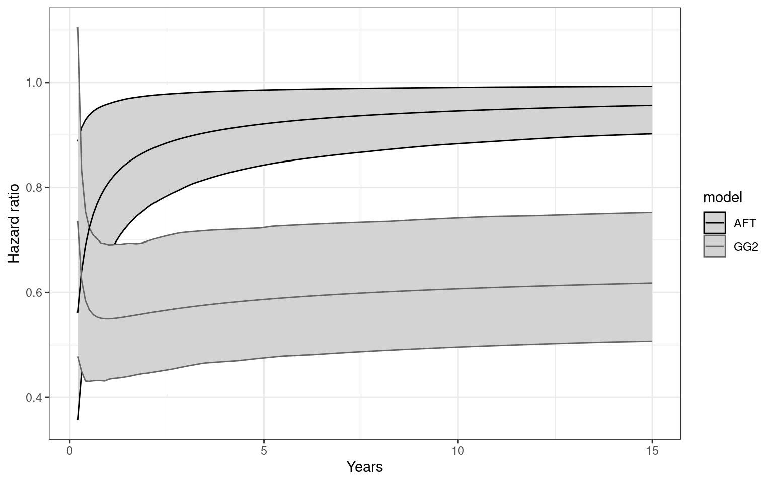
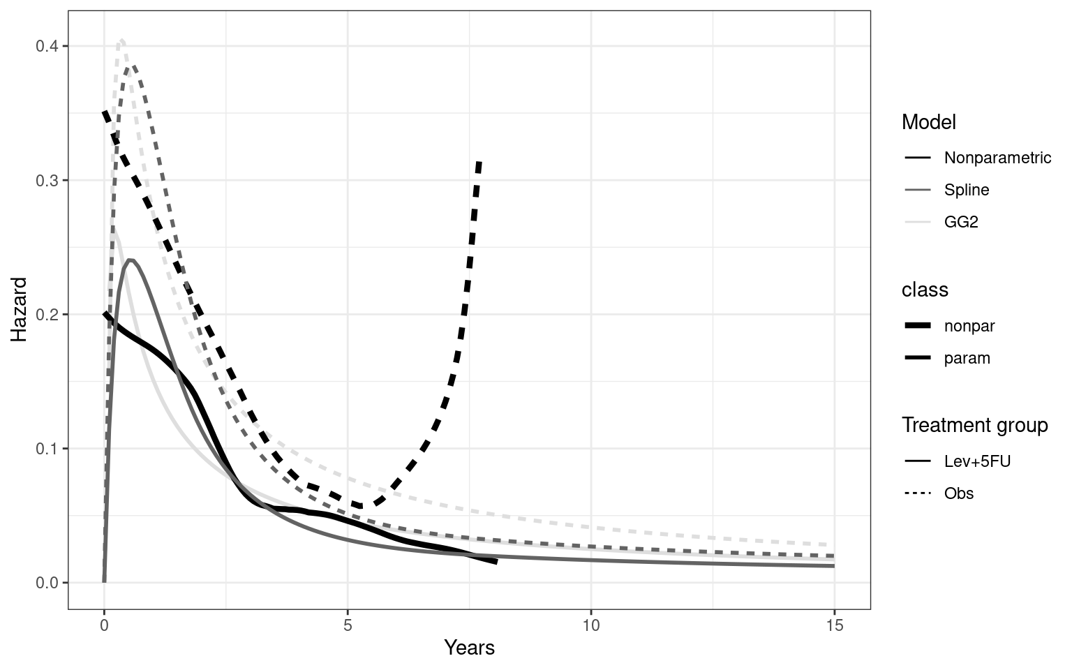
The PSM approach works effectively in estimating health state occupancy when the sample has been followed fully throughout the decision model’s time horizon. However, when the follow-up time in the studies that inform the OS and PFS probabilities are considerably less than the time horizon of the decision model, extrapolations are necessary for the OS and PFS probabilities. This is most often achieved through fitting parametric survival models to OS and PFS data using methods similar to those described above. However, given that OS and PFS are not independently defined, extrapolations from these parametric survival models and their subsequent application in PSMs can yield biased extrapolations. An extreme example of such inconsistency is when extrapolated PFS probabilities lie above the extrapolated OS probabilities, implicitly implying that a negative proportion of the cohort is occupying the progressed state. Therefore, modellers need to be careful in their considerations of the use of PSMs in decision modelling, especially when the data follow-up time is considerably smaller than the time horizon and/or when few events of the terminal health states (e..g death) have been observed. There is good documentation in the literature on the limitations of PSMs and the advantages of using state-transition and multi-state modelling as alternatives.

Achana, F.A., Cooper, N.J., Bujkiewicz, S., Hubbard, S.J., Kendrick, D., Jones, D.R., Sutton, A.J., 2014. Network meta-analysis of multiple outcome measures accounting for borrowing of information across outcomes. BMC Medical Research Methodology 14. https://doi.org/10.1186/1471-2288-14-92

Ades, A.E., 2003. A chain of evidence with mixed comparisons: models for multi-parameter synthesis and consistency of evidence. Statistics in Medicine 22, 2995–3016. https://doi.org/10.1002/sim.1566

Amdahl, J., 2022. Flexsurvcure: Flexible parametric cure models.

Baio, G., 2020. survHE: survival analysis for health economic evaluation and cost-effectiveness modeling. Journal of Statistical Software 95, 1–47.

Bucher, H.C., Guyatt, G.H., Griffith, L.E., Walter, S.D., 1997. The results of direct and indirect treatment comparisons in meta-analysis of randomized controlled trials. Journal of Clinical Epidemiology 50, 683–91. https://doi.org/10.1016/s0895-4356(97)00049-8

Che, Z., Green, N., Baio, G., 2023. Blended survival curves: A new approach to extrapolation for time-to-event outcomes from clinical trials in health technology assessment. Medical Decision Making 43, 299–310.

Cope, S., Chan, K., Jansen, J.P., 2020. Multivariate network meta-analysis of survival function parameters. Research Synthesis Methods 11, 443–456. https://doi.org/10.1002/jrsm.1405

Crowther, M.J., Lambert, P.C., 2014. A general framework for parametric survival analysis. Stat. Med. 33, 5280–5297.

Dias, S., Sutton, A.J., Ades, A.E., Welton, N.J., 2013. Evidence synthesis for decision making 2: A generalized linear modeling framework for pairwise and network meta-analysis of randomized controlled trials. Medical Decision Making 33, 607–17. https://doi.org/10.1177/0272989X12458724

Dziak, J.J., Coffman, D.L., Lanza, S.T., Li, R., Jermiin, L.S., 2019. Sensitivity and specificity of information criteria. Briefings in Bioinformatics 21, 553–565. https://doi.org/10.1093/bib/bbz016

Grafféo, N., Latouche, A., Le Tourneau, C., Chevret, S., 2019. ipcwswitch: An R package for inverse probability of censoring weighting with an application to switches in clinical trials. Computers in Biology and Medicine 111, 103339. https://doi.org/10.1016/j.compbiomed.2019.103339

Guyot, P., Ades, A., Ouwens, M.J., Welton, N.J., 2012. Enhanced secondary analysis of survival data: reconstructing the data from published Kaplan-Meier survival curves. BMC Medical Research Methodology 12. https://doi.org/10.1186/1471-2288-12-9

Hess, S. original by K., Gentleman, R. port by R., 2021. Muhaz: Hazard function estimation in survival analysis.

Hutton, B., Salanti, G., Caldwell, D.M., Chaimani, A., Schmid, C.H., Cameron, C., Ioannidis, J.P.A., Straus, S., Thorlund, K., Jansen, J.P., Mulrow, C., Catalá-López, F., Gøtzsche, P.C., Dickersin, K., Boutron, I., Altman, D.G., Moher, D., 2015. The PRISMA Extension Statement for Reporting of Systematic Reviews Incorporating Network Meta-analyses of Health Care Interventions: Checklist and Explanations. Annals of Internal Medicine 162, 777–784. https://doi.org/10.7326/m14-2385

Jackson, C., 2023. Survextrap: A package for flexible and transparent survival extrapolation. BMC Medical Research Methodology 23, 282.

Jackson, C., 2016. flexsurv: A Platform for Parametric Survival Modeling in R. Journal of Statistical Software 70. https://doi.org/10.18637/jss.v070.i08

Jackson, C., Stevens, J., Ren, S., Latimer, N., Bojke, L., Manca, A., Sharples, L., 2016. Extrapolating Survival from Randomized Trials Using External Data: A Review of Methods. Medical Decision Making 37, 377–390. https://doi.org/10.1177/0272989x16639900

Jansen, J.P., 2012. Network meta-analysis of individual and aggregate level data. Research Synthesis Methods 3, 177–90. https://doi.org/10.1002/jrsm.1048

Jansen, J.P., 2011. Network meta-analysis of survival data with fractional polynomials. BMC Medical Research Methodology 11, 61. https://doi.org/10.1186/1471-2288-11-61

Jansen, J.P., Fleurence, R., Devine, B., Itzler, R., Barrett, A., Hawkins, N., Lee, K., Boersma, C., Annemans, L., Cappelleri, J.C., 2011. Interpreting indirect treatment comparisons and network meta-analysis for health-care decision making: Report of the ISPOR task force on indirect treatment comparisons good research practices: Part 1. Value Health 14, 417–28. https://doi.org/10.1016/j.jval.2011.04.002

Kassambara, A., Kosinski, M., Biecek, P., 2021. Survminer: Drawing survival curves using ’ggplot2’.

Lambert, P.C., Thompson, J.R., Weston, C.L., Dickman, P.W., 2007. Estimating and modeling the cure fraction in population-based cancer survival analysis. Biostatistics 8, 576–594.

Latimer, N.R., 2013. Survival analysis for economic evaluations alongside clinical trials–extrapolation with patient-level data: Inconsistencies, limitations, and a practical guide. Med. Decis. Making 33, 743–754.

Latimer, N.R., Rutherford, M.J., 2024. Mixture and non-mixture cure models for health technology assessment: What you need to know. Pharmacoeconomics 42, 1073–1090.

Le Rest, K., Pinaud, D., Monestiez, P., Chadoeuf, J., Bretagnolle, V., 2014. Spatial leave-one-out cross-validation for variable selection in the presence of spatial autocorrelation. Global Ecology and Biogeography 23, 811–820. https://doi.org/10.1111/geb.12161

Liu, Xing-Rong, Pawitan, Y., Clements, M., 2018. Parametric and penalized generalized survival models. Stat. Methods Med. Res. 27, 1531–1546.

Liu, X.R., Pawitan, Y., Clements, M., 2018. Parametric and penalized generalized survival models 27, 1531–1546.

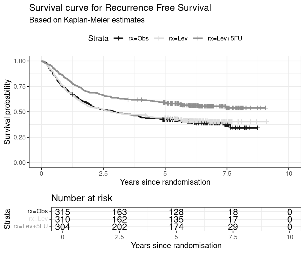
Moertel, C.G., Fleming, T.R., Macdonald, J.S., Haller, D.G., Laurie, J.A., Tangen, C.M., Ungerleider, J.S., Emerson, W.A., Tormey, D.C., Glick, J.H., Veeder, M.H., Mailliard, J.A., 1995. Fluorouracil plus levamisole as effective adjuvant therapy after resection of stage III colon carcinoma: a final report. Annals of Internal Medicine 122, 321–6. https://doi.org/10.7326/0003-4819-122-5-199503010-00001

Ouwens, M.J.N.M., Philips, Z., Jansen, J.P., 2010. Network meta-analysis of parametric survival curves. Research Synthesis Methods 1, 258–271. https://doi.org/10.1002/jrsm.25

Plummer, M., 2024. Rjags: Bayesian graphical models using MCMC.

Prentice, R., 1975. Discrimination among some parametric models. Biometrika 62, 607–614.

Royston, P., Parmar, M.K., 2013. Restricted mean survival time: An alternative to the hazard ratio for the design and analysis of randomized trials with a time-to-event outcome. BMC medical research methodology 13, 1–15.

Zhang, J.Z., Rios, J.D., Pechlivanoglou, T., Yang, A., Zhang, Q., Deris, D., Cromwell, I., Pechlivanoglou, P., 2024. SurvdigitizeR: an algorithm for automated survival curve digitization. BMC Medical Research Methodology 24. https://doi.org/10.1186/s12874-024-02273-8