| Study | Trt | \(r\) | \(n\) | Contamination level | Surgery type |
|---|---|---|---|---|---|
| Al-shehri 1994 | nonantibacterial | 7 | 134 | 1 | 0 |
| Al-shehri 1994 | antibiotic | 1 | 120 | 1 | 0 |
| Baker 1994 | nonantibacterial | 17 | 150 | 0 | 0 |
| Baker 1994 | antibiotic | 17 | 150 | 0 | 0 |
| Carl 2000 | nonantibacterial | 1 | 20 | 0 | 0 |
| $\ldots$ | $\ldots$ | $\ldots$ | $\ldots$ | $\ldots$ | $\ldots$ |
10 Network Meta-Analysis
Howard Z Thom
University of Bristol, UK
Nicky J Welton
University of Bristol, UK
David M Phillippo
University of Bristol, UK
Mathias Harrer
Technical University of Munich, Germany
10.1 Conceptual introduction to network meta-analysis
The topic of this chapter is network meta-analysis (NMA). This is the primary method for indirect treatment comparison recommended by the International Society for Pharmacoeconomics and Outcomes Research (ISPOR), society for Medical Decision Making (SMDM), UK National Institute for Health and Care Excellence (NICE), German Gemeinsamer Bundesausschuss (GBA), and European Joint Clinical Assessments (JCA) (Dias et al., 2011 (last updated September 2016); G-BA, 2011; Hoaglin et al., 2011; HTA CG, 2024; Jansen et al., 2011). It has been placed at the top of the evidence hierarchy by international experts in evidence synthesis, and has been used by the World Health Organization (WHO) in their guidelines (Kanters et al., 2016; Leucht et al., 2016). Hundreds of NMAs have been published to date (Efthimiou and White, 2020).
10.1.1 Motivation for network meta-analysis
Double-blind randomised controlled trials (RCTs) are the gold standard for estimating relative treatment effects (Hariton and Locascio, 2018). RCTs randomise patients to two or more treatment arms. One arm is usually a control, which can be a placebo or active intervention. Randomization aims to balance patient characteristics so the treatment effect estimates are not biased by systematic differences in prognostic factors (Zabor et al., 2020). In a double-blind RCT, patients, clinicians, and assessors are furthermore blinded to intervention allocation, minimising possible bias. However, head-to-head RCTs comparing treatments of interest are not always available.
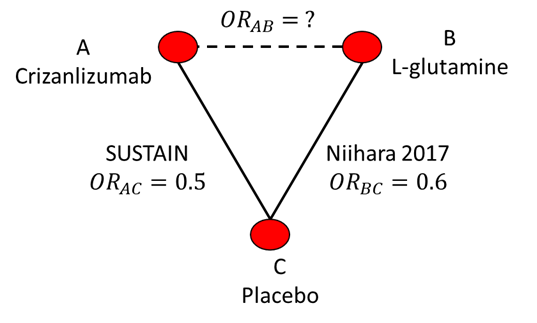
As an example, consider a published NMA of Sickle Cell Disease (SCD) and treatments for the prevention of vaso-occlusive pain crises (Thom et al., 2020a). The SUSTAIN (NCT01895361) RCT has compared crizanlizumab to placebo while the Niihara 2017 (NCT01179217) RCT compared L-glutamine to placebo (Ataga, 2017; Niihara, 2017). There was no head-to-head RCT that directly compared crizanlizumab to L-glutamine. The evidence network is illustrated in Figure 10.1. NMA provides a way to indirectly compare these treatments for pain crisis prevention that preserves the randomisation and blinding of RCTs.
10.1.2 The Bucher method
Suppose SUSTAIN reported an odds ratio for crizanlizumab (treatment A) vs placebo (treatment C) on pain crisis prevention of 0.5 and that Niihara (2017) reported an odds ratio for L-glutamine (treatment B) vs placebo on crisis prevention of 0.6. We can use direct RCT evidence comparing treatment A with C and B with C to indirectly compare A with B. Note that we refer to A vs C or B vs C as a treatment contrast or comparison.
An approach to indirect comparison was proposed by Bucher et al. (1997) They suggested that the odds ratio for A vs B can be calculated as \[ \text{OR}_{AB}= \frac{\text{OR}_{AC}}{\text{OR}_{BC}} \] \[ \text{OR}_{AB} = \frac{0.5}{0.6} = 0.83 \] We can also write the relationship on the log odds scale \[ \log(\text{OR}_{AB})= log(\text{OR}_{AC}) - log(\text{OR}_{BC}) \] This is the linear predictor scale as treatment effects are additive. This scale also clarifies how the standard errors of log odds ratios can be calculated if correlation is assumed to be zero
\[ \text{se}_{AB}= \sqrt{\text{se}_{AC}^2 + \text{se}_{BC}^2} \]
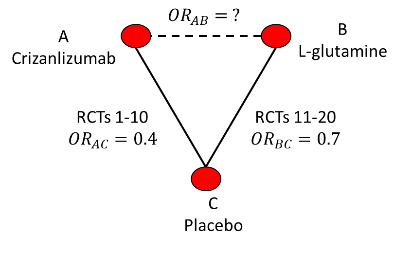
A simple generalisation is to the scenario where multiple RCTs are available on each comparison. Then the \(\text{OR}_{AC}\) and \(\text{OR}_{BC}\) could be assumed to be the results of a meta-analysis. If the results were as in Figure 10.2 then the estimate would again be \(\text{OR}_{AB}=\frac{0.4}{0.7}=0.57\).
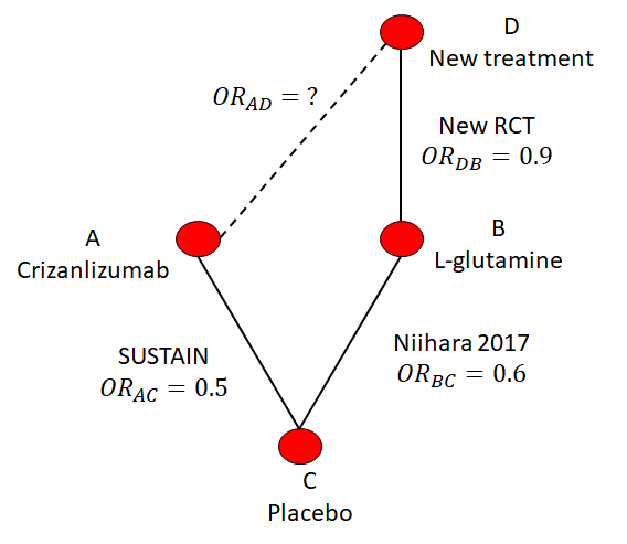
Suppose there were some new treatment D that is compared to L-glutamine in a new RCT. The hypothetical network is illustrated in Figure 10.3. This new RCT reports an odds ratio of 0.9 (so better than L-glutamine) but it’s unknown how it compares to crizanlizumab. The Bucher method would be applied in steps (i.e., In Figure 10.3 first from A to C, then from C to B, and finally from B to D) to indirectly compare the new treatment with crizanlizumab.
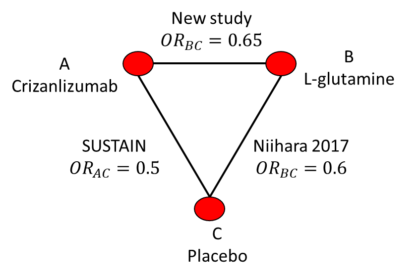
A final consideration is Figure 10.4 where we now have both direct and indirect evidence with which to compare crizanlizumab and L-glutamide. In this case we have a study that estimated their odds ratio to be \(\text{OR}_{AB}=0.65\). We could meta-analyse this direct odds ratio with the indirect odds ratio from Bucher but this motivates the need for a more general method for combining direct and indirect evidence on multiple nodes and with multiple studies on each edge.
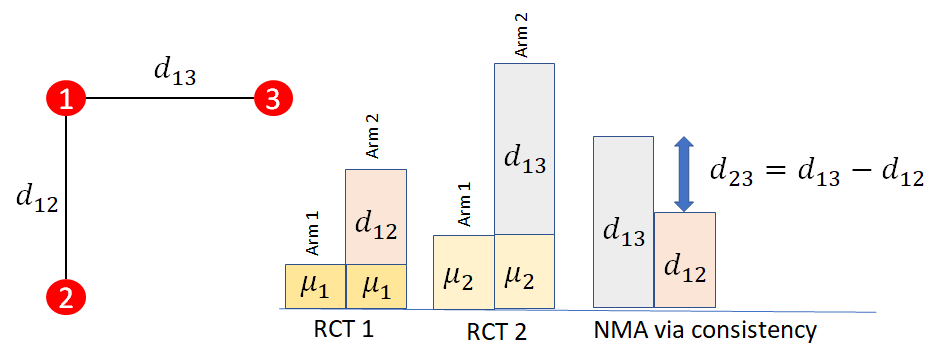
10.1.3 NMA and the consistency assumption
Network meta-analysis is an indirect comparison method that builds on a fully generalised Bucher with multiple RCTs on each contrast (e.g., as in Figure 10.2) and network geometry (e.g., as in Figure 10.3) to also allow both direct and indirect evidence on comparisons e.g., as in 10.4. It also estimates the uncertainty (i.e. standard errors) from meta-analysing multiple RCTs and indirect comparison. NMA uses the consistency assumption, which loosely means that relative treatment effects, such as log odds ratios in the SCD example, can be added to give the correct relative treatment effect (Lumley, 2002). Generally, NMA is conducted on the linear predictor scale, which again is the scale on which treatment effects are additive. In the SCD example, this means that NMA would operate on log odds ratios rather than directly on the odds ratio scale.
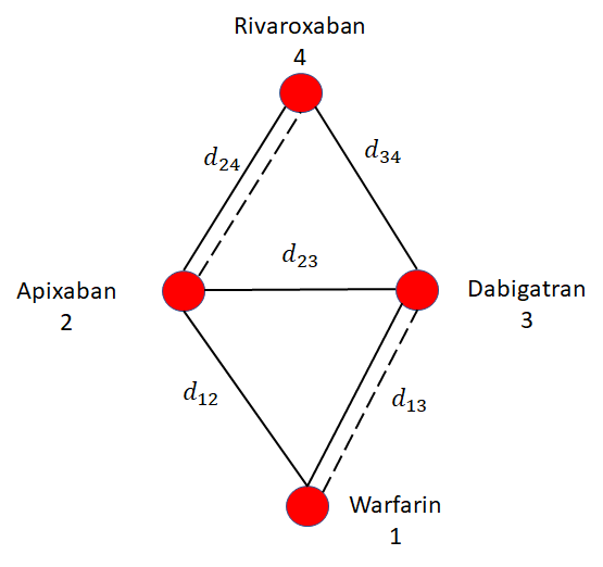
The consistency assumption is illustrated in Figure 10.5. In this illustration, it is assumed that there is only one RCT comparing treatments 2 vs 1 (with relative treatment effect \(d_{12}\)) and one RCT comparing 3 vs 1 (with relative treatment effect \(d_{13}\). The baseline effects \(\mu_{i}\) represent the (for example) log odds of event on the baseline treatment of trial \(i\). These cancel out when estimating the log odds ratios \(d_{12}\) and \(d_{13}\). Consistency tells us that the effect of treatment 3 vs 2 is calculated by \[d_{23} = d_{13} - d_{12}\]
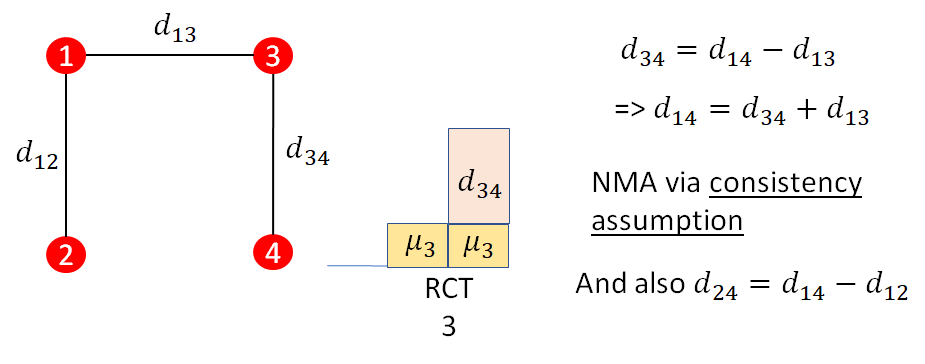
A further illustration of the consistency assumption is provided in Figure 10.6. In this case, there is a further RCT comparing treatment 4 to treatment 3 (\(d_{34}\)). This treatment effect is related to the previous effects relative to treatment 1 via consistency: \[d_{34}=d_{14}-d_{13}\] In general NMA is relating all relative effects \(d_{xy}\) to the basic parameters \(d_{1x}\) and \(d_{1y}\), which are treatment effects relative to treatment 1. Treatment 1 is named the reference treatment and consistency in general is: \[d_{xy} = d_{1y} - d_{1x}\]
10.1.4 NMA on binary outcomes - the binomial logistic model
We have so far explained the theory for how the relative treatment effects \(d_{xy}\) relate to each other through consistency, but not how they are related to the data.
Binary outcomes data consist of \(r_{ik}\) events out of \(n_{ik}\) patients on treatment \(t_{ik}\) in each arm \(k\) of study \(i\). For example, in a RCT on treatments for prevention of stroke in atrial fibrillation, this could be 10 patients with a stroke in 200 patients on the warfarin arm and 5 patients with stroke in 190 patients on the apixaban arm.
We will use a binomial likelihood \[r_{ik}\sim \text{Binomial}(p_{ik}, n_{ik}) \] Where \(p_{ik}\) is the probability of having the event. This probability is bounded between 0 and 1 and probabilities are not additive, which makes modelling difficult. We therefore use a link function to map the probability to a scale with range \((-\infty, \infty)\), on which we can assume treatment effects are additive. The logistic link function provides such a transformation: \[\text{logit}(p) = \log\left(\frac{p}{1-p}\right) \] The resulting scale is the log odds scale and differences in log odds are log odds ratios. Applying this to our model of binary outcomes gives \[ \text{logit}(p_{ik}) = \mu_{i} + \delta_{i,bk}\] The \(b\) is the baseline or control arm of the trial and is always \(b=1\) (i.e., first arm though not necessarily first treatment as \(t_{ib}\) does not need to be \(1\)). The \(\delta_{i,bk}\) are the trial specific log odds ratios for the treatment in arm \(k\) compared to that in arm \(b\), so \(\delta_{i,bb}=0\) by definition.
The final step is to relate study specific log odds ratios \(\delta_{i,bk}\) between treatments in study arms to the log odds ratios relative to treatment 1 (i.e., \(d_{1x}\)).
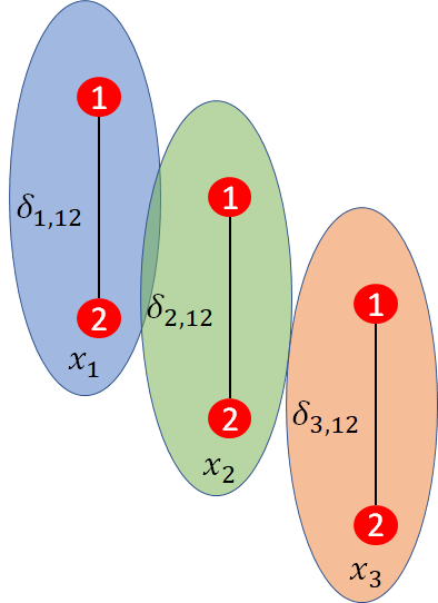
To do this we specify if we are assuming fixed effects across studies or random effects across studies (Borenstein et al., 2010). Under fixed effects, also known as common effects, the relative treatment effects are assumed to be the same across studies. This gives us \(\delta_{i, bk}=d_{t_{ib}t_{ik}}\) where \(t_{ib}\) and \(t_{ik}\) are the treatments in arm \(b\) and \(k\), respectively, of trial \(i\). Furthermore, applying the consistency assumption \[\delta_{i, bk}=d_{1 t_{ik}} - d_{1 t_{ib}} \] Where the \(1\) is the reference treatment of the evidence network. Under random effects, the study specific log odds ratios are assumed to vary Normally around the \(d_{t_{ib}t_{ik}}\) giving \[\delta_{i, bk} \sim \text{Normal}(d_{1 t_{ik}} - d_{1 t_{ib}}, \sigma^2) \] where the \(\sigma^2\) is the heterogeneity variance.
Heterogeneity refers to the extent of variation between studies and in meta-analysis and NMA commonly refers to variation in treatment effects across studies (Deeks et al., 2023). Choice between fixed and random effects should be guided by an assessment of the extent this heterogeneity. This includes considering the similarity of baseline characteristics, outcome definitions, timepoints, concomitant treatments, and other elements of study design. Greater heterogeneity suggests that random effects may be more appropriate. The choice can also be informed by statistical assessments of model fit, which are explained shortly. Comparing the estimated heterogeneity standard deviation \(\sigma\) to the estimated log odds ratios \(d_{1x}\) gives an assessment of the heterogeneity relative to the size of the treatments; if \(\sigma\) is much greater than the log odds ratios then heterogeneity may affect the ability to draw conclusions from the analysis. Relatively larger \(\sigma\) suggests that random effects should be selected. The estimated variance could also be compared to published heterogeneity variances on similar interventions, related diseases and comparable outcomes, giving a measure of “high” or “low” heterogeneity (Salanti et al., 2014).
10.1.5 Bayesian and frequentist estimation
NMA can be conducted using either Bayesian or frequentist estimation (Sadeghirad et al., 2023) — see Chapter 4 for more details on different approaches to statistical inference. Under the Bayesian paradigm parameters such as treatment effects (\(d_{1x}\)) are viewed as random variables that have probability distributions. These distributions represent our beliefs about the parameters, updating our prior beliefs with the observed evidence from the data. Under the frequentist paradigm, by contrast, it is assumed that parameters are fixed but unknown. Distributions instead represent sampling uncertainty in their estimates. Estimates are calculated by, for example, finding the values of \(d_{1x}\) and \(\sigma\) that maximise the likelihood of the observed data.
In Bayesian statistics we assign a prior distribution to each unknown parameter. For treatment effects relative to the reference treatment (i.e., treatment 1) in NMA this could be a highly vague or uncertain distribution \[ d_{1x} \sim \text{Normal}(0, 10^6) \] If using random effects the heterogeneity standard deviation prior could be \[ \sigma \sim \text{Uniform}(0, 5) \] Both of these priors are vague, as they are very uncertain with respect to treatment effects measured as log odds ratios, standardised mean differences or log hazard ratios, although they may need adjustment for other outcomes. Informative priors could be used in NMA to represent clinical opinion on treatment effects or the extent of heterogeneity. For random effects models, it is possible to use published informative priors on the heterogeneity standard deviation (Rhodes et al., 2016).
Note that the definition of a prior as vague or informative depends on the scale on which the treatment effects are measured; for example, the above uniform prior for the heterogeneity standard deviation \(\sigma\) would not be vague for treatment effects measured in kilograms of body weight.
We then update our beliefs about the parameters using the data, as represented by the likelihood. After updating, we have posterior distributions on the \(d_{1x}\) and, under random effects, \(\sigma\).
Interpretation of results also depends on the selected method for estimation. In frequentist statistics, a 95% confidence interval (CI) is calculated for the estimated treatment effects \(\hat{d}_{1x}\). This interval is the range which would contain the true \(d_{1x}\) 95% of the time if we resampled and recalculated the CI. We test hypotheses that, for example, the \(d_{1x}\) are different from zero. p-values represent the probability of observing the data (e.g., under binomial data the \(r_{ik}\) and \(n_{ik}\)), or something more extreme, if the null hypothesis is true. P-values are often interpreted at the 5% significance threshold (i.e., if the p-value is below 0.05 the null hypothesis can be rejected) but more generally the lower the p-value the stronger the evidence against the null hypothesis.
In Bayesian statistics, we can summarise our findings using the estimated posterior distributions. A 95% credible interval (CrI) for \(d_{1x}\) is the range in which we have a 95% belief that it contains the true \(d_{1x}\). If this 95% CrI excludes the \(d_{1x}\) that corresponds to no effect (e.g., a log odds ratio of \(0\), mean difference of \(0\), or rate ratio of \(1\)) then we can interpret it to indicate evidence of a difference between treatment \(x\) and \(1\). Conversely, if the 95% CrI includes the no effect value then we interpret it to mean there is no evidence of a difference. We don’t have p-values but can calculate the probability that, for example, each \(d_{1x}\) is above 0. In binomial-logistic model this would be the probability that the log odds ratio of the event is higher on treatment than on control (so treatment is better if an event is good, or worse if an event is bad). This Bayesian p-value could be interpreted in a similar way to a one-sided frequentist p-value (Spiegelhalter et al., 2004).
R packages exist to fit NMA under both the frequentist and Bayesian paradigm. In this chapter, we will present the multinma package for Bayesian estimation and netmeta for frequentist estimation. Other Bayesian options include gemtc or interfacing with an external Bayesian estimator through R2OpenBUGS, R2WinBUGS, rjags or rstan (Carpenter et al., 2017; Lunn et al., 2013; Plummer et al., 2003; Team, 2023). The frequentist meta-analysis package metafor can also be used for NMA (Viechtbauer, 2010).
10.1.6 Bayesian statistical assessments of model performance and fit
There are a variety of tools used to assess the fit and performance of NMA models in both the frequentist and Bayesian setting. In the Bayesian setting, the absolute fit of a model is commonly assessed using the residual deviance (Dias et al., 2013a; McCullagh and Nelder, 1989). The residual deviance measures the difference between model predictions and actual observations. The residual deviance for the binomial model is \[ D_{res}=\sum_{i}\sum_{k}2\left( r_{ik} \log\left(\frac{r_{ik}}{\hat{r}_{ik}}\right) +(n_{ik} - r_{ik}) \log\left(\frac{n_{ik}-r_{ik}}{n_{ik}- \hat{r}_{ik} }\right)\right) \] \[ = \sum_{i}\sum_{k}dev_{ik} \] where \(\hat{r}_{ik}=n_{ik}p_{ik}\) is the expected number of events. The posterior mean residual deviance (\(\bar{D}_{res}\)) is compared to the number of observations (number of arms across all trials). The posterior mean residual deviance (\(\bar{dev}_{ik}\)) for individual observations can be inspected to see where fit is worst.
The Deviance Information Criterion (DIC) is a Bayesian model assessment criterion that gives an measure of model performance by trading off fit (deviance) and complexity (effective number of parameters) (Spiegelhalter et al., 2002) \[ \text{DIC} = D_{res} + p_{D} \] with lower DIC values being desirable. Differences of 5 or more are considered important, but this is not a solid rule with advice on meaningful differences ranging from 3 to 7 (Lunn et al., 2013).
10.1.7 Frequentist statistical assessments of model performance and fit
In the frequentist NMA implementation we cover here, important model diagnostics can be derived from \(Q_{\text{total}}\), which measures the total heterogeneity/inconsistency in the network (Deeks et al., 2023; Higgins et al., 2003). These measures are also helpful to decide if a fixed-effect or random-effects model is more appropriate.
\(Q_{\text{total}}\) is a generalised version of Cochran’s \(Q\), which is often calculated in “conventional” meta-analyses to test the between-study heterogeneity. It is defined as follows:
\[Q_{\text{total}}:= (\boldsymbol{d}-\hat{\boldsymbol{\delta}}^{\text{NMA}})^\top \boldsymbol{W}(\boldsymbol{d}-\hat{\boldsymbol{\delta}}^{\text{NMA}})\]
In this equation, \(\boldsymbol{d}=(d_i, \dots, d_m)^\top\) are the \(i, \dots, m\) effect sizes (e.g., log odds ratios) included in our dataset, and \(\hat{\boldsymbol{\delta}}^{\text{NMA}}\) are the treatment effect estimates we obtained via a (frequentist) network meta-analysis. The letter \(\boldsymbol{W}\) stands for a matrix whose diagonal elements include the inverse-variance weights \((1/s^2_i, \dots, 1/s^2_m)\) of the \(m\) treatment comparisons in our data, which are assumed to be known.
When there is no heterogeneity, this total heterogeneity statistic \(Q_{\text{total}}\) is assumed to follow a \(\chi^2\) distribution with degrees of freedom \(\nu\) equal to \(\left(\sum_k p_k-1\right)-(n-1)\). Here, \(p_k\) is the number of arms included in some study \(k\), and \(n\) is the total number of treatments in the network. This can be used to perform a \(Q\)-test, indicating if there is significant excess variability in our data. It also allows to derive a version of the \(I^2\) statistic that generalises to network meta-analytic models (Higgins et al., 2003; Higgins and Thompson, 2002)
\[I^2=\text{max}\left\{\frac{Q_{\text{total}}-\nu}{Q_{\text{total}}},0\%\right\} \]
Similar to pairwise meta-analyses, \(I^2\) is bounded between 0% and 100%. Higher values indicate a higher amount of heterogeneity/inconsistency in our model. Along with other indicators, large \(I^2\) values may indicate that a random-effects model may be more appropriate for our NMA. However, it has been noted that the \(I^2\) does not indicate possible ranges of the treatment effect in future studies and thus may not be a sensible quantification of heterogeneity (M. et al., 2017).
There are also other diagnostics that can be derived from \(Q_{\text{total}}\), which can be used to locate specific designs that increase the heterogeneity/inconsistency in our model. We will cover these later in this chapter.
10.1.8 Network meta-regression
When there are is heterogeneity or inconsistency in treatment effects, network meta-regression may be used to attempt to explain this variation in relative treatment effects between studies based on measured covariates (Dias et al., 2013b). Suppose we are conducting a pairwise meta-analysis of three trials, as illustrated in Figure 10.7. This could be comparing the efficacy of a new intervention to Warfarin on prevention of stroke in atrial fibrillation.
The treatment effect between treatments \(2\) and \(1\) is \(d_{12}\), which would be the log odds ratio. Now suppose that the mean age of patients in trial \(i\) is \(x_{i}\) and that this varies between trials. Age is very likely to be a prognostic factor as older patients are at greater risk of stroke. However, it may also be a treatment effect modifier so trial specific treatment effects \(\delta_{i, 12}\) will be related to \(x_{i}\). For example, younger patients may respond better to treatment or vice versa.
Only treatment effect modifiers are of concern to NMA, since prognostic factors are cancelled out within studies by randomisation.
In pairwise meta-analysis, a simple meta-regression model can be written as \[\delta_{i,12}=d_{12}+x_{i}\beta \] where \(x_{i}\) is a trial specific baseline characteristic (e.g. age, duration of disease, severity) and \(\beta\) is a regression coefficient that needs to be estimated. Note that \(\beta\) is not identifiable if there are fewer than two trials on the treatment contrast. If \(d_{12}\) is a log odds ratio, the \(\beta\) would be the amount the log odds ratio increases for each unit increase in \(x_{i}\), so \(\exp(\beta)\) is an odds ratio of odds ratios.
To extend our binomial-logistic NMA into a network meta-regression model we change the link function equations for probability \(p_{ik}\) to include a regression term \[ \text{logit}(p_{ik}) = \mu_{i} + (\delta_{i,bk} + x_{ik}\beta_{i, bk})\] The \(x_{ik}\) is the trial and arm specific value of the covariate while \(\beta_{i, bk}\) is the (trial dependent) treatment-by-covariate interaction term given by another set of consistency equations \[ \beta_{i,bk}= \beta_{t_{ik}} - \beta_{t_{ib}}\] We will make the common assumption that \(\beta_{1}=0\) so that only effects relative to control/placebo are affected. This is necessary for star-shaped networks and helpful for otherwise limited networks.
Various assumptions are possible on the remaining treatment specific regression coefficients \(\beta_{z}\) where \(z \ne 1\). We could assume separate and unrelated interaction terms for each treatment so that each \(\beta_{z}\) is different and independent. We could also assume exchangeable (random effects) interaction terms across treatments: \[ \beta_{z} \sim \text{Normal}(B, \sigma_{\beta}) \] Finally, we could also assume a common or shared interaction terms across treatments: \[ \beta_{2}=\ldots=\beta_{n_{t}}=B \] This last assumption is most likely to be useful due to limited evidence on effect modifiers but it is a very strong assumption. NMAs often have only small numbers of trials on each contrast. An established rule-of-thumb is that 10 trials, with a good spread in values of the covariate, are needed to somewhat reliably estimate a covariate effect but networks rarely have this many trials on any of the contrasts. As for the choice of fixed or random effects, the choice of whether to include a covariate can be informed using statistical assessments (e.g., DIC and residual deviance). However, it is important to be guided by clinical opinion and qualitative assessment on the extent of imbalance in potential effect modifiers.
10.1.9 Statistical tests for inconsistency
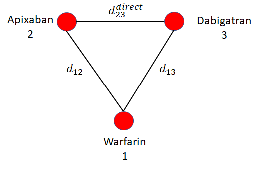
Consider the example evidence network in Figure 10.8 comparing treatments for stroke prevention in atrial fibrillation. In this hypothetical illustration, there is be a loop of trials comparing apixaban, dabigatran, and warfarin. The consistency assumption of NMA implies that indirect estimate of effect of apixaban relative to dabigatran \[ d^{\rm{indirect}}_{23} = d_{13}-d_{12} \] is the same as would be observed in a trial directly comparing apixaban and dabigatran (\(d^{\rm{direct}}_{23}\)).
However, if treatment effect modifiers are different in the trials informing \(d_{13}\) and \(d_{12}\) to that estimating \(d^{direct}_{23}\) then perhaps \[ d^{\rm{direct}}_{23} \ne d^{\rm{indirect}}_{23} \] This is called inconsistency, sometimes also called incoherence (Dias et al., 2018, 2013c). Inconsistency and heterogeneity are closely linked, and are both caused by differences in treatment effects between studies: inconsistency is variation in treatment effects between studies on different comparisons, heterogeneity is variation in treatment effects between studies on the same comparison. Testing for inconsistency is possible whenever there is a loop of evidence as in Figure 10.8, but inconsistency is always possible in NMA even when it cannot be tested.
The first approach to testing inconsistency we will consider is the inconsistency model or unrelated mean effects (UME) model. The UME model removes the usual consistency assumption and instead treats all treatment contrasts \(d_{ck}\) (for treatments \(c\) and \(k\)) as independent so, for example, we would have \[ d_{ck} \ne d_{1k} - d_{1c} \] This model can be fit and its DIC and total residual deviance compared to the consistency model. Substantially lower DIC or residual deviance in the UME model indicates inconsistency is present. If a random effects model is fitted, then a reduction in heterogeneity in the UME model also indicates that inconsistency is present. This provides a global test for inconsistency but does not indicate the evidence loops in which inconsistency is likely to be present.
A local test for inconsistency is provided by node splitting. Node splitting separates the direct and indirect evidence on a single edge in each evidence loop. In the example network of Figure 10.9, node splitting could estimate posterior distributions to compare \[ d^{\rm{indirect}}_{13} \text{ vs } d^{\rm{direct}}_{13} \] and \[ d^{\rm{indirect}}_{24} \text{ vs } d^{\rm{direct}}_{24} \] The choice of edge on which to test in each loop is arbitrary and results would be similar we compared, say, \(d_{24}\), \(d_{34}\), or \(d_{23}\) in the first loop or \(d_{12}\), \(d_{13}\) or \(d_{23}\) in the second. Specific results may be affect by priors in Bayesian analysis or properties of the estimation procedure in either Bayesian or frequentist analysis.
Comparing 95% CI or CrI on the direct and indirect estimates (or estimating p-values for differences) tests for inconsistency. This is a local test for inconsistency and highlights problematic loops.
Similar methods can also be applied in a frequentist framework to diagnose network inconsistency. An alternative approach, which is used by the frequentist NMA implementation we will cover in this chapter, puts greater emphasis on the variability between designs in a network (Jackson et al., 2014). The advantage of this approach is that it is uniquely specified but with the disadvantage that it can be unintuitive and gives an overspecified model.
It is important to remember that, in a conventional pairwise meta-analysis, all studies have the same design (e.g., they compare treatment A to treatment B). This means that all trials provide direct evidence for one specific comparison (A vs. B), and within this design, effects can be more or less heterogeneous. In NMA, we include various designs (e.g., studies comparing A with B; B with C; or multi-arm trials comparing A, B and C, and so forth), and this can additionally lead to inconsistency in effects between the different designs.
We have previously introduced \(Q_{\text{total}}\), which quantifies the total amount of heterogeneity and inconsistency in our network. It is possible to break down \(Q_{\text{total}}\) into its two components: the heterogeneity of effects within the same designs (\(Q_{\text{het}}\)), and inconsistency of effects between different designs (\(Q_{\text{inc}}\)) (Krahn et al., 2013):
\[Q_{\text{total}} = Q_{\text{het}} + Q_{\text{inc}} \]
When there is no inconsistency, the \(Q_{\text{inc}}\) statistic is assumed to follow a \(\chi^2\) distribution with \(\left(\sum_d (p_d-1)\right)-(n-1)\) degrees of freedom, where \(p_d\) is the number of arms in a specific design \(d\). This can be used perform a test of the overall inconsistency in our model.
The between-design variability \(Q_{\text{inc}}\) can also be further decomposed. This allows to inspect which specific designs mainly contribute to the inconsistency in our network. It is also possible to recalculate the statistic after specific designs have been removed (“detached”). If the recalculated \(Q\) value after detaching a specific design is considerably lower, this indicates that much of the inconsistency is caused by that particular design. As we will see in the applied example, individual inconsistency contributions of each design can also be visualised in a “net heat plot”. Such graphs also allow to find “hot spots” of inconsistency in which the evidence of several designs do not support each other.
Tests of the (detached) \(Q_{\text{inc}}\) values assume a fixed-effect model. It is also possible to examine the residual inconsistency when assuming a “design-by-treatment interaction” random effects model. This is a type of random-effects model with additional parameters to incorporate network inconsistency via design-by-treatment interactions (i.e., they allow the model to capture additional effect variability between designs, beyond the normal between-study heterogeneity). Later in this chapter, we will see this approach in practice.
10.2 The surgical site infection example
Our working example is a published NMA of irrigation and intracavity lavage (ICL) techniques to prevent Surgical Site Infections (SSIs, Thom et al., 2020b). SSIs are wound infections that occur after an operative procedure (Perencevich et al., 2003). They are costly and associated with poorer patient outcomes, increased mortality, morbidity and reoperation rates. Surgical wound ICL are intraoperative techniques, which may reduce the rate of SSIs through removal of dead or damaged tissue, metabolic waste, and wound exudate.
The NMA on SSI was published in 2021 and was on 42 RCTs with 11,726 participants. In this published NMA, antibiotic classes were split into four categories (i.e. Cephalosporin, penicillin, aminoglycoside, and other) but we merge them for simplicity. As a result, we exclude 3 studies that compared one antibiotic to another (Mohd et al., 2010; Peterson et al., 1990; Trew et al., 2011). This leaves the example with 39 RCTs and 10,997 patients. In addition to antibiotic irrigation, the interventions are nonantibacterial irrigation, no irrigation, and antiseptic irrigation. The data are the number of patients with an SSI in each arm of each trial. The reference treatment is nonantibacterial irrigation. The data are stored in the R object icl_data_long which is presented below. In this table, presented in long format with a row for each arm of each study, trt is the treatment name, r is the number of SSIs in each arm, n is the number of patients in each arm, while the two binary covariates are contamination_level (0 if clean and 1 if contaminated, dirty or mixed) and surgery_type (1=abdominal, 2=surgery with prostheses).
10.3 Bayesian NMA using the multinma package
The first R package we will explore is multinma. This is a package of functions for Bayesian NMA implemented using the Stan software.
library(multinma)
# To set up parallel processing
options(mc.cores = parallel::detectCores())
To get a better idea of the evidence, we first explore the evidence network implied by the icl_data_long dataset. To do this we use the set_agd_arm() function to create a network object from the data which are in the format of aggregate data on each study arm (i.e. event counts and sample sizes on each arm). Note that for the meta-regression we will conduct later, we need all non-nonantibacterial treatments in a common class and thus specify the trt_class argument.
icl_network <- set_agd_arm(
  icl_data_long,
  study = study,
  trt = trt,
  r = r,
  n = n,
  trt_class = as.numeric(trt != "nonantibacterial")
)

# Print a summary of the network
icl_network
A network with 39 AgD studies (arm-based).
------------------------------------------------------- AgD studies (arm-based) ----
Study Treatment arms
Al-shehri 1994 2: nonantibacterial | antibiotic
Baker 1994 2: nonantibacterial | antibiotic
Carl 2000 2: nonantibacterial | antibiotic
Case 1987 2: nonantibacterial | antibiotic
cervantes-sanchez 2000 2: nonantibacterial | no irrigation
Cheng 2005 2: nonantibacterial | antiseptic
cho 2004 2: nonantibacterial | no irrigation
Dashow 1986 2: nonantibacterial | antibiotic
de jong 1982 2: antiseptic | no irrigation
elliott 1986 2: antibiotic | no irrigation
... plus 29 more studies
Outcome type: count
------------------------------------------------------------------------------------
Total number of treatments: 4, in 2 classes
Total number of studies: 39
Reference treatment is: nonantibacterial
Network is connectedPrinting the network object icl_network gives us some useful information about the network. This includes the number of studies, the type of outcome (i.e. count), the total number of treatments and classes (i.e. 4 and 2, respectively), and tests if the network is connected. A network would be disconnected if a treatment could not be compared to nonantibacterial irrigation through a direct or indirect path of studies.
We can also illustrate the evidence network using the plot() function below. Each node represents a treatment and edges represent studies comparing the corresponding treatments. Node size is related to the number of patients on the treatment (included using the weight_nodes argument) while edge thickness is related to the number of studies on the comparison (included with the weight_edges argument).
plot(icl_network, weight_nodes = TRUE, weight_edges = TRUE)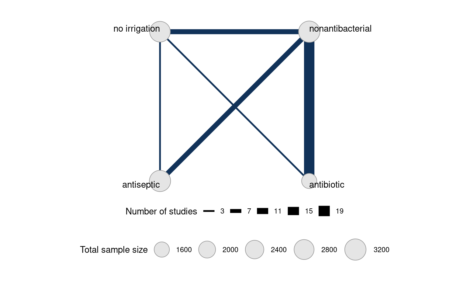
Fitting either fixed or random effects network meta-analyses are accomplished using the nma() function. The trt_effects argument can be set to "fixed" or "random" to specify fixed or random effects, respectively. Prior distributions on the \(\mu_{i}\) and \(d_{ix}\) are specified using the prior_intercept and prior_trt arguments. In our example we set them to normal(scale = 100) so they have a mean of zero and, as specified by the scale argument, a standard deviation of 100. For random effects only, a prior on the heterogeneity standard deviation \(\sigma\) is specified using prior_het and, in our example, set to a half-Normal distribution with half_normal(scale = 2.5).
icl_fit_fe <- nma(icl_network,
                  trt_effects = "fixed",
                  prior_intercept = normal(scale = 100),
                  prior_trt = normal(scale = 100))

icl_fit_re <- nma(icl_network,
                trt_effects = "random",
                prior_intercept = normal(scale = 100),
                prior_trt = normal(scale = 100),
                prior_het = half_normal(scale = 2.5))
Basic summaries are given using the print() commmand. We see that Rhat is close to 1 under both models (less than 1.05 is acceptable), meaning that convergence is achieved.
print(icl_fit_fe)A fixed effects NMA with a binomial likelihood (logit link).
Inference for Stan model: binomial_1par.
4 chains, each with iter=2000; warmup=1000; thin=1;
post-warmup draws per chain=1000, total post-warmup draws=4000.
mean se_mean sd 2.5% 25% 50% 75% 97.5%
d[antibiotic] -0.76 0.00 0.13 -1.01 -0.85 -0.76 -0.68 -0.51
d[antiseptic] -0.33 0.00 0.12 -0.57 -0.41 -0.33 -0.24 -0.09
d[no irrigation] -0.14 0.00 0.13 -0.40 -0.22 -0.14 -0.05 0.11
lp__ -3239.35 0.12 4.70 -3249.36 -3242.34 -3238.91 -3236.07 -3231.33
n_eff Rhat
d[antibiotic] 5214 1
d[antiseptic] 2545 1
d[no irrigation] 2603 1
lp__ 1520 1
Samples were drawn using NUTS(diag_e) at Thu Jun 5 20:17:30 2025.
For each parameter, n_eff is a crude measure of effective sample size,
and Rhat is the potential scale reduction factor on split chains (at
convergence, Rhat=1).print(icl_fit_re)A random effects NMA with a binomial likelihood (logit link).
Inference for Stan model: binomial_1par.
4 chains, each with iter=2000; warmup=1000; thin=1;
post-warmup draws per chain=1000, total post-warmup draws=4000.
mean se_mean sd 2.5% 25% 50% 75% 97.5%
d[antibiotic] -0.83 0.00 0.22 -1.26 -0.98 -0.82 -0.68 -0.41
d[antiseptic] -0.58 0.01 0.28 -1.15 -0.75 -0.56 -0.39 -0.06
d[no irrigation] -0.04 0.01 0.27 -0.57 -0.22 -0.04 0.14 0.49
lp__ -3235.74 0.22 7.95 -3252.25 -3240.90 -3235.30 -3230.29 -3221.03
tau 0.66 0.00 0.16 0.38 0.54 0.64 0.76 1.02
n_eff Rhat
d[antibiotic] 2089 1
d[antiseptic] 1550 1
d[no irrigation] 1818 1
lp__ 1261 1
tau 1352 1
Samples were drawn using NUTS(diag_e) at Thu Jun 5 20:17:37 2025.
For each parameter, n_eff is a crude measure of effective sample size,
and Rhat is the potential scale reduction factor on split chains (at
convergence, Rhat=1).To help choose between fixed and random effects, we can look at the DIC. Residual deviance and DIC are considerably lower on the random effects model. Given our prior expectation of heterogeneity in the network, we select the random effects model for analysis.
(icl_dic_fe <- dic(icl_fit_fe))Residual deviance: 138.9 (on 80 data points)
pD: 43.2
DIC: 182.1(icl_dic_re <- dic(icl_fit_re))Residual deviance: 86.8 (on 80 data points)
pD: 60.5
DIC: 147.3We can also inspect individual study and arm residual deviances. The plot below suggests Cheng (2005) antiseptic and Kubota (2015) antiseptic fit poorly. This is unsurprising given they are both zero-event arms.
plot(icl_dic_re)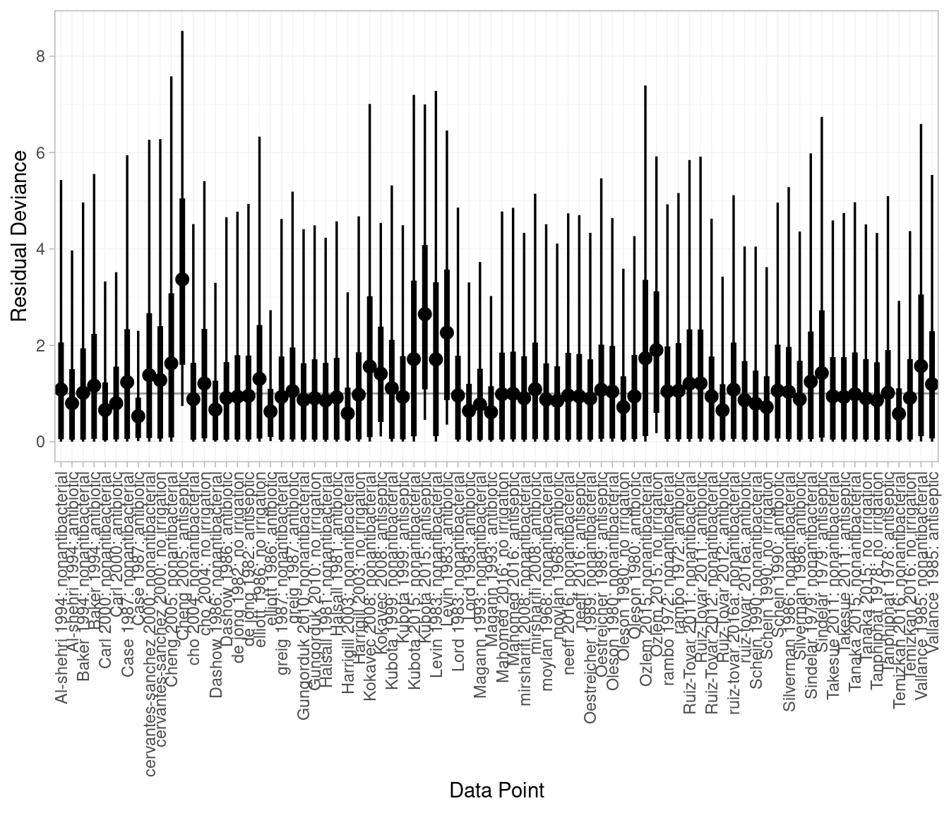
Once we are satisfied the models have converged, have chosen between fixed and random effects, and assessed the fit of the models, we can look at the relative effect estimates. In multinma we can compute relative effects against our reference treatment, in this case nonantibacterial irrigation, using the relative_effects() function. These are provided on the linear predictor scale, in this case log odds ratios, but can be exponentiated to the odds ratio scale.
(icl_relative_effects_re <- relative_effects(
  icl_fit_re, trt_ref = "nonantibacterial"
))
mean sd 2.5% 25% 50% 75% 97.5% Bulk_ESS Tail_ESS Rhat
d[antibiotic] -0.83 0.22 -1.26 -0.98 -0.82 -0.68 -0.41 2120 2613 1
d[antiseptic] -0.58 0.28 -1.15 -0.75 -0.56 -0.39 -0.06 1654 2137 1
d[no irrigation] -0.04 0.27 -0.57 -0.22 -0.04 0.14 0.49 1834 2684 1# Store as an array and exponentiate from log odds ratios to odds ratios
lor_array <- as.array(icl_relative_effects_re)
or_array <- exp(lor_array)
(icl_or_re <- summary(or_array)) mean sd 2.5% 25% 50% 75% 97.5% Bulk_ESS Tail_ESS Rhat
d[antibiotic] 0.45 0.10 0.28 0.38 0.44 0.51 0.67 2120 2613 1
d[antiseptic] 0.58 0.16 0.32 0.47 0.57 0.67 0.95 1654 2137 1
d[no irrigation] 1.00 0.27 0.56 0.80 0.96 1.15 1.63 1834 2684 1These results can be plotted using the plot() function, i.e. plot(icl_relative_effects_re) to plot the log odds ratios, or plot(icl_or_re) to plot the odds ratios. To create a forest plot with the estimates tabulated alongside the graphical summaries, we can use the forestplot() function of the forestplot package. We can see that the antibiotic and antiseptic irrigation have odds ratios below 1.00 and their 95% CrI do not overlap with 1.00, which we interpret as there being evidence of lower SSI rates on these interventions than on nonantibacterial irrigation. The odds ratio for no irrigation is very close to 1.00 and its 95% CrI overlaps with 1.00, which we interpret as there being no evidence of a difference in SSI rates between this intervention and nonantibacterial irrigation.
icl_or_re_forest <- as.data.frame(icl_or_re)
icl_or_re_forest$estci <- sprintf("%.2f (%.2f, %.2f)",
                                  icl_or_re_forest$mean,
                                  icl_or_re_forest$`2.5%`,
                                  icl_or_re_forest$`97.5%`)

forestplot::forestplot(icl_or_re_forest,
                       mean = mean, lower = `2.5%`, upper = `97.5%`,
                       labeltext = c(parameter, estci),
                       boxsize = .1,
                       # Axis ticks on log scale
                       xlog = TRUE)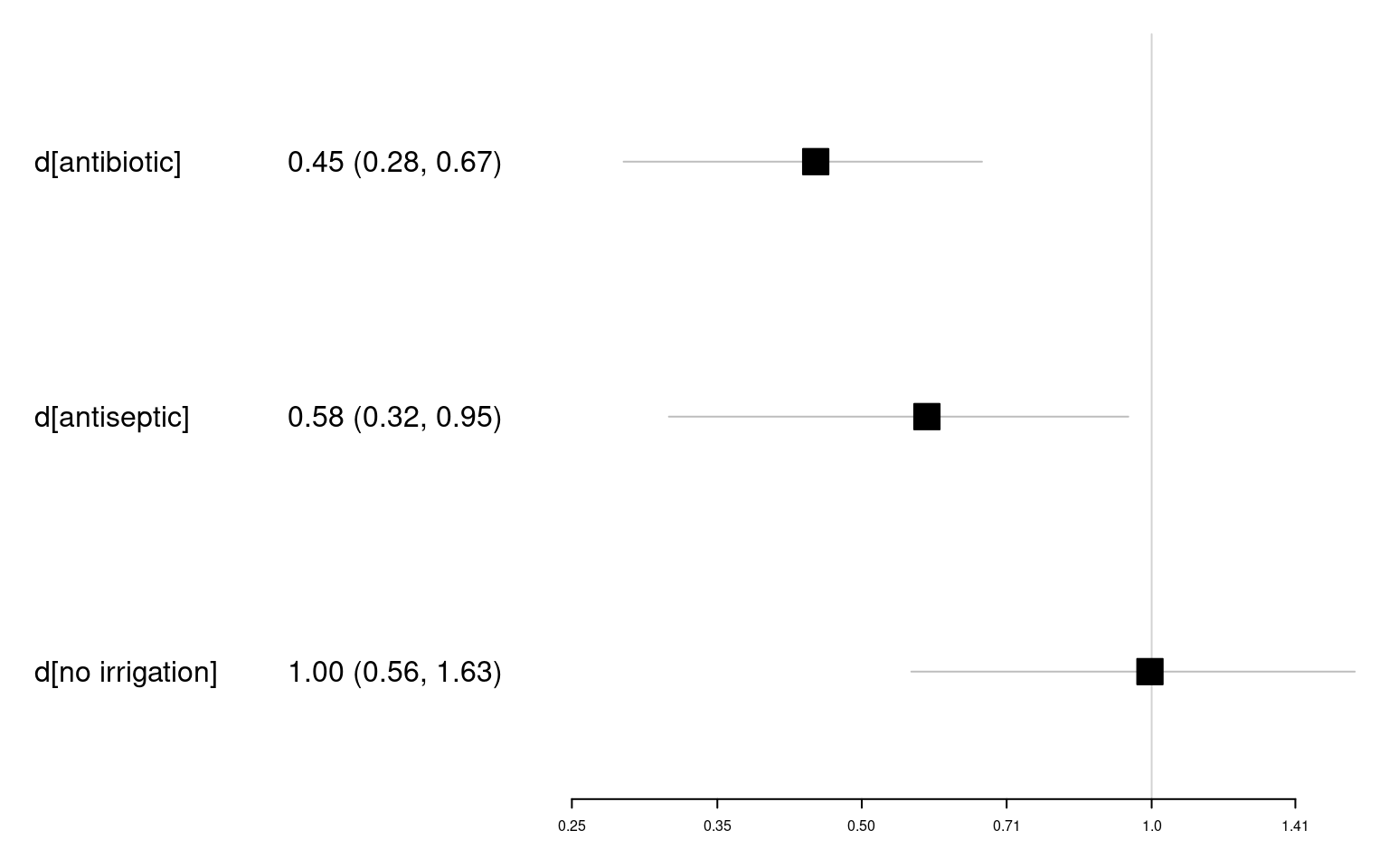
In addition to comparisons with nonantibacterial irrigation and other pairwise comparisons, it would be helpful to understand how the treatments are performing overall. In NMA this is commonly achieved using treatment rankings. Using multinma we can use posterior_ranks() function to estimate ranks and posterior_rank_probs() to estimate probabilities of having each rank. The output of posterior_rank_probs() can be plotted using plot() to generate a rankogram.
# Mean ranks and other summary statistics
(icl_ranks_re <- posterior_ranks(icl_fit_re))
mean sd 2.5% 25% 50% 75% 97.5% Bulk_ESS Tail_ESS Rhat
rank[nonantibacterial] 3.54 0.53 3 3 4 4 4 2233 NA 1
rank[antibiotic] 1.24 0.45 1 1 1 1 2 2312 2317 1
rank[antiseptic] 1.82 0.51 1 2 2 2 3 2381 2350 1
rank[no irrigation] 3.40 0.58 2 3 3 4 4 2360 NA 1# Probability of occupying each rank
(icl_probs_re <- posterior_rank_probs(icl_fit_re)) p_rank[1] p_rank[2] p_rank[3] p_rank[4]
d[nonantibacterial] 0.00 0.01 0.43 0.55
d[antibiotic] 0.77 0.22 0.01 0.00
d[antiseptic] 0.23 0.73 0.04 0.01
d[no irrigation] 0.00 0.04 0.52 0.44# Plot the rankogram
plot(icl_probs_re)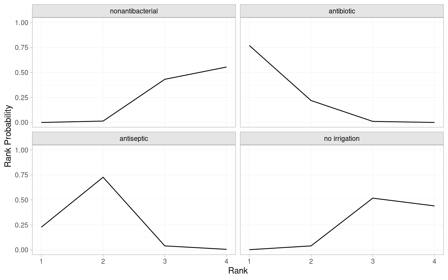
The mean ranks indicate that antibiotic irrigation is ranked first (mean rank of 1.24 is closest to 1.00) and antiseptic is second (mean rank of 1.82). Conversely, no irrigation and nonantibacterial irrigation are ranked 3rd or 4th. The probabilities of occupying each rank suggest antibiotic has the greatest probability (0.77) of ranking 1st and antiseptic has greatest probability (0.73) of ranking 2nd. The rankograms illustrate this visually. An interpretative shorthand is that a “flat” rankogram indicates uncertainty about which rank is occupied by an intervention, while a “spikey” rankogram indicates confidence that a treatment occupies one or more ranks. In the SSI NMA, the antibiotic and antiseptic rankograms are spikey as there is a high probability they are ranked 1st or 2nd, respectively. Conversely, the nonantibacterial and no irrigation rankgrams are flat over 3rd and 4th ranks, suggesting uncertainty about which intervention is actually the worst at preventing SSIs.
Cumulative ranking probabilities can be generated by setting cumulative = TRUE in posterior_rank_probs() and a plot of this output is called a cumulative rankogram.
# Cumulative probabilities of occupying each rank
(icl_cum_probs_re <- posterior_rank_probs(icl_fit_re, cumulative = TRUE))
p_rank[1] p_rank[2] p_rank[3] p_rank[4]
d[nonantibacterial] 0.00 0.01 0.45 1
d[antibiotic] 0.77 0.99 1.00 1
d[antiseptic] 0.23 0.95 0.99 1
d[no irrigation] 0.00 0.04 0.56 1# Plot the cumulative rankograms
plot(icl_cum_probs_re)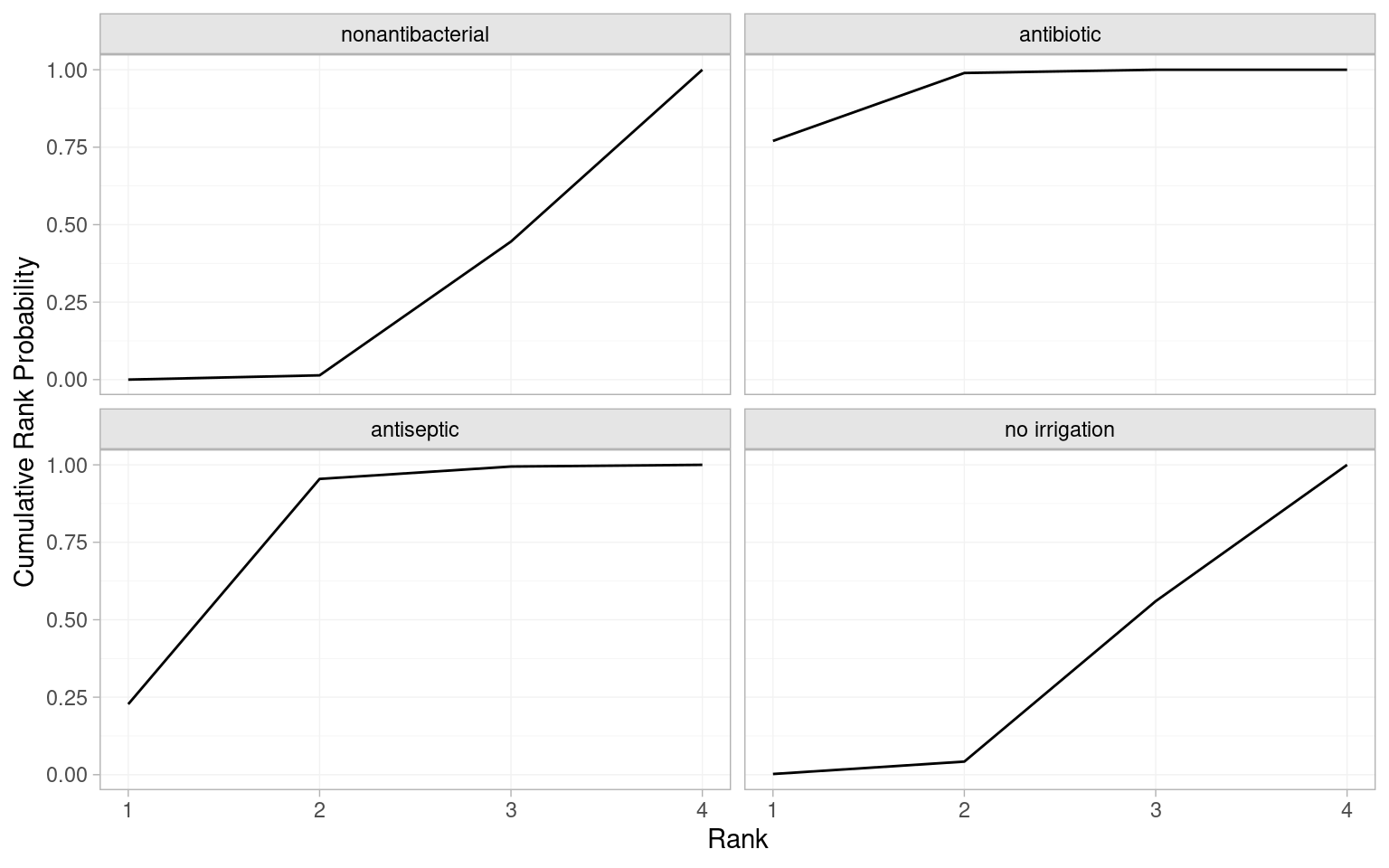
Contamination level (named contamination_level) was reported by all the included studies, and is 1 if contaminated, dirty or mixed, and 0 if clean. As this is a potential treatment effect modifier, it is important to attempt a network meta-regression. Meta-regression is also implemented using the nma() function but with the additional regression argument to specify the regression formula for the covariate or covariates, class_interactions to specify the relationship between regression coefficients, and prior_reg to specify a prior for the regression coefficient(s). To maximise statistical power, we assume a common regression coefficient across the three non-reference interventions (i.e., the three that are not nonantibacterial).
icl_fit_re_contamination <- nma(icl_network,
                                trt_effects = "random",
                                regression = ~.trt:contamination_level,
                                class_interactions = "common",
                                prior_intercept = normal(scale = 100),
                                prior_trt = normal(scale = 100),
                                prior_reg = normal(scale = 100),
                                prior_het = half_normal(scale = 2.5))
# Inspect the regression coefficients and model fit statistics
print(icl_fit_re_contamination)A random effects NMA with a binomial likelihood (logit link).
Regression model: ~.trt:contamination_level.
Centred covariates at the following overall mean values:
contamination_level
0.45
Inference for Stan model: binomial_1par.
4 chains, each with iter=2000; warmup=1000; thin=1;
post-warmup draws per chain=1000, total post-warmup draws=4000.
mean se_mean sd 2.5% 25% 50%
beta[.trtclass1:contamination_level] 0.22 0.01 0.32 -0.41 0.00 0.21
d[antibiotic] -0.83 0.00 0.22 -1.27 -0.98 -0.83
d[antiseptic] -0.60 0.01 0.29 -1.22 -0.77 -0.59
d[no irrigation] -0.05 0.01 0.28 -0.61 -0.22 -0.05
lp__ -3235.50 0.25 7.97 -3252.19 -3240.63 -3235.18
tau 0.68 0.01 0.17 0.39 0.56 0.66
75% 97.5% n_eff Rhat
beta[.trtclass1:contamination_level] 0.42 0.85 1924 1
d[antibiotic] -0.69 -0.39 2135 1
d[antiseptic] -0.41 -0.06 1546 1
d[no irrigation] 0.12 0.50 1875 1
lp__ -3229.89 -3220.67 985 1
tau 0.78 1.05 1111 1
Samples were drawn using NUTS(diag_e) at Thu Jun 5 20:17:49 2025.
For each parameter, n_eff is a crude measure of effective sample size,
and Rhat is the potential scale reduction factor on split chains (at
convergence, Rhat=1).dic(icl_fit_re_contamination)Residual deviance: 86.5 (on 80 data points)
pD: 61.1
DIC: 147.6The regression coefficient (beta[.trtclass1:contamination_level]) has a posterior mean of 0.22 and 95% CrI (-0.41, 0.85) suggesting no evidence of effect modification. Furthermore, the residual deviance is similar to the unadjusted random effects NMA (86.5 vs 86.8), as is the DIC (147.6 vs 147.3), again suggesting no improvement in model fit or performance from including the regression. The estimate of the heterogeneity standard deviation tau is also unchanged. We could conclude that our analysis is robust to potential effect modification by contamination level, although it’s important to recall that aggregate data meta-regressions are underpowered. Individual patient data meta-regression on contamination level could tell a different story.
Our final consideration is if there is any evidence of inconsistency. As seen in Figure 10.10 there are two loops of studies where we can compare the direct and indirect estimates. The first approach is to fit an unrelated mean effects model to the ICL network, which is again done using the nma() function but with the additional argument consistency = "ume". One technical point related to estimation is that we increase the maximum tree depth using control = list(max_treedepth = 15) to avoid warning messages, caused by the very small amount of data on the antibiotic vs no irrigation comparison making this harder to estimate; this is not generally necessary. We then compare the DIC of the inconsistency model to our base case consistency model.
# Testing inconsistency using an unrelated mean effects (inconsistency) model
icl_fit_re_ume <- nma(icl_network,
                      consistency = "ume",
                      trt_effects = "random",
                      prior_intercept = normal(scale = 100),
                      prior_trt = normal(scale = 100),
                      prior_het = normal(scale = 2.5),
                      # Increase max_treedepth to avoid warnings
                      control = list(max_treedepth = 15))
The total residual deviance of the inconsistency model is very similar to that of consistency model (86.1 vs 86.8), as is the DIC (146.7 vs 147.3). The heterogeneity estimate has decreased slightly under the UME model.
# Compare the DIC and residual deviance to the consistency model
(icl_dic_re_ume <- dic(icl_fit_re_ume))
Residual deviance: 86.1 (on 80 data points)
pD: 60.6
DIC: 146.7(icl_dic_re)Residual deviance: 86.8 (on 80 data points)
pD: 60.5
DIC: 147.3It is important to compare the residual deviance contributions for each data point, between the usual NMA consistency model and the inconsistency UME model. We do this graphically by calling plot() on the two dic objects.
plot(icl_dic_re, icl_dic_re_ume, show_uncertainty = FALSE)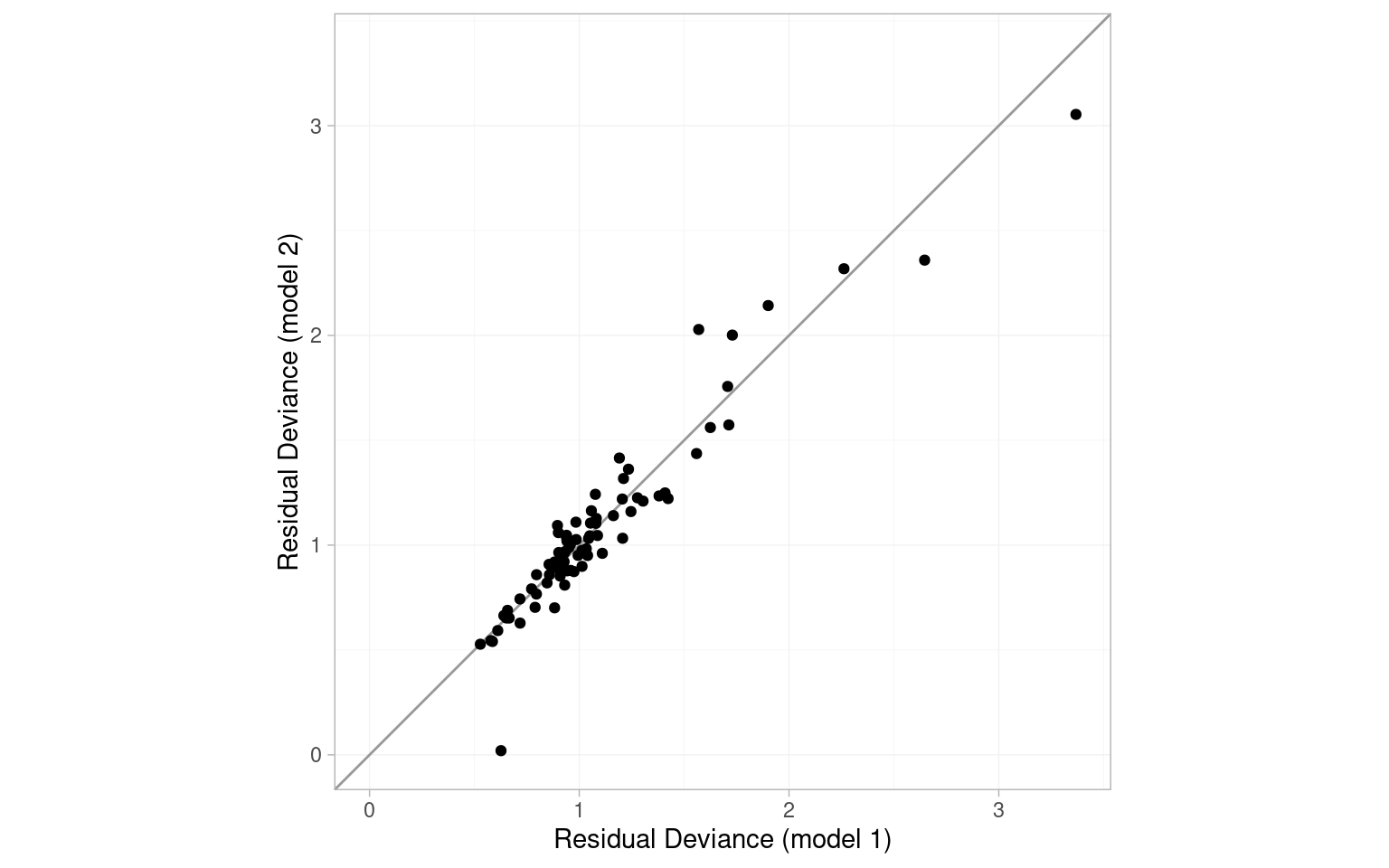
The points are scattered around the line of equality, and in particular there are no points lying in the lower-right portion of the plot that would have poor fit under the consistency model but good fit under the UME model. Overall, there is little evidence for inconsistency based on the UME model.
The second approach to testing inconsistency is node splitting. The nma() function with argument consistency = "nodesplit" will automatically detect independent loops of evidence and compare direct and indirect estimates of relative treatment effects.
# Testing for inconsistency using node splitting
icl_fit_re_nodesplit <- nma(icl_network,
                            consistency = "nodesplit",
                            trt_effects = "random",
                            prior_intercept = normal(scale = 100),
                            prior_trt = normal(scale = 100),
                            prior_het = half_normal(scale = 2.5),
                            # Increase max_treedepth to avoid warnings
                            control = list(max_treedepth = 15))
The results of the node splitting models are then summarised with the summary() function.
# Summarise nodesplits
summary(icl_fit_re_nodesplit)
Node-splitting models fitted for 5 comparisons.
------------------------------------ Node-split antibiotic vs. nonantibacterial ----
mean sd 2.5% 25% 50% 75% 97.5% Bulk_ESS Tail_ESS
d_net -0.82 0.22 -1.26 -0.96 -0.82 -0.67 -0.39 1775 2153
d_dir -0.81 0.22 -1.25 -0.95 -0.81 -0.66 -0.37 2763 2436
d_ind -56.16 41.90 -157.44 -81.21 -47.91 -22.96 -2.24 1978 2331
omega 55.35 41.91 1.38 22.09 47.05 80.41 156.61 1980 2331
tau 0.66 0.16 0.38 0.55 0.65 0.76 1.03 1344 1760
tau_consistency 0.66 0.16 0.40 0.55 0.64 0.75 1.00 1254 2311
Rhat
d_net 1
d_dir 1
d_ind 1
omega 1
tau 1
tau_consistency 1
Residual deviance: 85.9 (on 80 data points)
pD: 60.7
DIC: 146.7
Bayesian p-value: 0.021
------------------------------------ Node-split antiseptic vs. nonantibacterial ----
mean sd 2.5% 25% 50% 75% 97.5% Bulk_ESS Tail_ESS Rhat
d_net -0.58 0.27 -1.16 -0.75 -0.57 -0.40 -0.06 1756 2139 1
d_dir -0.86 0.32 -1.51 -1.06 -0.85 -0.65 -0.27 2746 2659 1
d_ind 0.25 0.51 -0.74 -0.08 0.23 0.56 1.30 1665 1865 1
omega -1.11 0.60 -2.37 -1.48 -1.08 -0.71 0.04 1680 2222 1
tau 0.62 0.17 0.33 0.50 0.60 0.72 1.00 1256 2145 1
tau_consistency 0.66 0.16 0.40 0.55 0.64 0.75 1.00 1254 2311 1
Residual deviance: 86.5 (on 80 data points)
pD: 60.4
DIC: 146.8
Bayesian p-value: 0.059
--------------------------------- Node-split no irrigation vs. nonantibacterial ----
mean sd 2.5% 25% 50% 75% 97.5% Bulk_ESS Tail_ESS Rhat
d_net -0.04 0.28 -0.58 -0.23 -0.04 0.14 0.48 1793 2531 1.00
d_dir 0.23 0.32 -0.40 0.02 0.23 0.43 0.85 2814 3174 1.00
d_ind -0.72 0.48 -1.69 -1.03 -0.71 -0.41 0.21 1477 1755 1.00
omega 0.95 0.57 -0.19 0.57 0.95 1.32 2.11 1607 1913 1.00
tau 0.62 0.17 0.33 0.50 0.61 0.72 0.97 1086 1914 1.01
tau_consistency 0.66 0.16 0.40 0.55 0.64 0.75 1.00 1254 2311 1.00
Residual deviance: 87.2 (on 80 data points)
pD: 60.1
DIC: 147.3
Bayesian p-value: 0.093
--------------------------------------- Node-split no irrigation vs. antibiotic ----
mean sd 2.5% 25% 50% 75% 97.5% Bulk_ESS Tail_ESS Rhat
d_net 0.77 0.34 0.10 0.55 0.77 1.00 1.43 1944 2429 1
d_dir 0.97 0.65 -0.28 0.52 0.96 1.39 2.27 2721 2716 1
d_ind 0.74 0.38 0.01 0.48 0.72 0.98 1.52 1626 2013 1
omega 0.23 0.71 -1.12 -0.25 0.22 0.69 1.68 1876 2347 1
tau 0.68 0.17 0.39 0.56 0.66 0.78 1.07 1029 1747 1
tau_consistency 0.66 0.16 0.40 0.55 0.64 0.75 1.00 1254 2311 1
Residual deviance: 86.7 (on 80 data points)
pD: 61.7
DIC: 148.4
Bayesian p-value: 0.76
--------------------------------------- Node-split no irrigation vs. antiseptic ----
mean sd 2.5% 25% 50% 75% 97.5% Bulk_ESS Tail_ESS Rhat
d_net 0.54 0.31 -0.05 0.33 0.52 0.73 1.18 2118 2732 1
d_dir 0.02 0.41 -0.78 -0.24 0.02 0.28 0.82 2882 2582 1
d_ind 1.12 0.44 0.30 0.83 1.11 1.40 2.02 1720 2094 1
omega -1.10 0.60 -2.33 -1.48 -1.09 -0.70 0.09 1569 1948 1
tau 0.63 0.17 0.34 0.51 0.61 0.73 1.00 1221 2101 1
tau_consistency 0.66 0.16 0.40 0.55 0.64 0.75 1.00 1254 2311 1
Residual deviance: 86.2 (on 80 data points)
pD: 60.3
DIC: 146.5
Bayesian p-value: 0.065Across the node split comparisons, there are no notable drops in residual deviance or DIC compared to consistency model, while heterogeneity was only very slightly lower for some comparisons. However, there were some small Bayesian p-values, notably antibiotic vs. nonantibacterial (p-value of 0.021), no irrigation vs antiseptic (0.065) and antiseptic vs nonantibacterial (0.059), suggesting inconsistency may be a concern.
We can also use the plot() function to visually compare the direct, indirect and NMA estimates. As expected given the low p-values, the antiseptic vs nonantibacterial and no irrigation vs antiseptic comparisons have greater separation between direct and indirect estimates. The indirect evidence on the antibiotic vs. nonantibacterial comparison is very uncertain, and the NMA estimate for this comparison is driven entirely by the direct evidence.
# Plot direct and indirect estimates
plot(icl_fit_re_nodesplit) +
  theme(legend.position=c(.85,.2))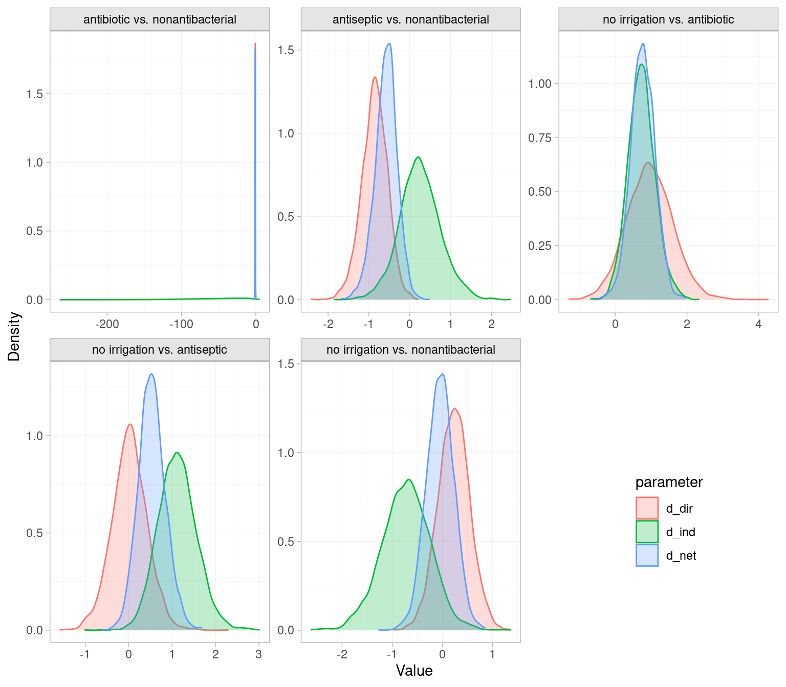
10.4 Frequentist NMA using the netmeta package
We have shown above how to conduct an NMA under the Bayesian paradigm but will now repeat much of the analysis using the frequentist package netmeta.
library(netmeta)There is some data cleaning required to get the ICL evidence into the format expected by netmeta. We first load the data in a format with matrices r, n, and t for the numbers of events, numbers of patients, and numbers of treatments. These each have a row for each study and column for each arm. The number of columns is set to 3 as this is the largest number of arms per single study (the Oleson 1980 and Schein 1990 studies have 3 arms each). Furthermore, netmeta does not accept independent arms on the same treatment within each trial, so we merge the relevant r and n to obtain a single arm. netmeta does accept strings as the treatment names so replace the numeric codes with meaningful names.
# Load the icl_data list with matrices r, n and t for events, patients, and
# treatments, and the vector na with number of arms per study.
load("data/icl_data.rda")
t_names <- c("nonantibacterial",  "no irrigation",  "antiseptic",  "antibiotic")

# Netmeta does not accept independent arms on the same treatment within a trial
# Need to merge arms on the same treatment
for(i_study in 1:icl_data$ns) {
  # Which treatments are studied in this study?
  study_treatments <- unique(icl_data$t[i_study, ])
  for(i_treatment in study_treatments[!is.na(study_treatments)]) {
    # Index the arms on this treatment
    arm_index <- icl_data$t[i_study, ] == i_treatment
    arm_index[is.na(arm_index)] <- FALSE
    if(sum(arm_index) > 1) {
      # Merge to just one arm on this treatment
      icl_data$t[i_study, arm_index] <-
        c(i_treatment, rep(NA, sum(arm_index) - 1))
      icl_data$na[i_study] <- icl_data$na[i_study] - sum(arm_index) + 1
      # r and n are the sum of events and patients across all arms
      icl_data$r[i_study, arm_index] <-
        c(sum(icl_data$r[i_study, arm_index]), rep(NA, sum(arm_index) - 1))
      icl_data$n[i_study, arm_index] <-
        c(sum(icl_data$n[i_study, arm_index]), rep(NA, sum(arm_index) - 1))
    }
  }
}

# Netmeta can take strings as the treatment names
temp <- matrix("", dim(icl_data$t)[1], dim(icl_data$t)[2])
rownames(temp) <- rownames(icl_data$t)
for(i_study in 1:dim(temp)[1]) {
  temp[i_study, ] <- t_names[icl_data$t[i_study, ]]
}
icl_data$t <- temp
With that, we can call the netmeta::pairwise() function to transform the data from arm-base format to contrast-based format. This calculates odds ratios in each trial relative to the reference. This function automatically adds a continuity correction of 0.5 to any arms with zero events. Table 10.2 shows the first few rows of the computed values for ORs and their standard error.
# Transform data from arm-based format to contrast-based format
# Studlab is repeated for studies with >2 arms (e.g. Oleson 1980 with 3 arms)
icl_network <- pairwise(treat = list(t[, 1], t[, 2], t[, 3]),
                        event = list(r[, 1], r[, 2], r[, 3]),
                        n = list(n[, 1], n[, 2], n[, 3]),
                        data = icl_data, sm = "OR",
studlab = names(na))| TE | seTE | studlab | treat1 | treat2 |
|---|---|---|---|---|
| 1.881 | 1.077 | Al-shehri 1994 | nonantibacterial | antibiotic |
| 0 | 0.364 | Baker 1994 | nonantibacterial | antibiotic |
| 0 | 1.451 | Carl 2000 | nonantibacterial | antibiotic |
| 0.871 | 1.656 | Case 1987 | nonantibacterial | antibiotic |
| -1.257 | 0.366 | cervantes-sanchez 2000 | nonantibacterial | no irrigation |
| $\ldots$ | $\ldots$ | $\ldots$ | $\ldots$ | $\ldots$ |
Fitting a fixed effects NMA is accomplished via the netmeta() function, which takes as input the treatment effects, standard errors, treatment labels, and study labels from the icl_network object. The netmeta() function fits both a fixed and random effects model but arguments can be passed to only output fixed or random effects. The arguments common = TRUE and random = FALSE specify that a fixed effect model be output, with netmeta referring to fixed effects as common effects. Conversely setting common = FALSE and random = TRUE outputs a random effects model.
# Output the results of a fixed effects NMA
icl_fit_fe <- netmeta(TE, seTE, treat1, treat2, studlab, data = icl_network,
                      common = TRUE, random = FALSE,
                      reference.group = "nonantibacterial")

# Output the results of a random effects NMA
icl_fit_re <- netmeta(TE, seTE, treat1, treat2, studlab, data = icl_network,
                      common = FALSE, random = TRUE,
                      reference.group = "nonantibacterial")
We can print the results of these analyses and use summary statistics to compare fixed and random effects. The \(I^2\) being 46.6% and low p-value (0.0032) for tests of within designs heterogeneity again favour a random effects analysis.
icl_fit_feNumber of studies: k = 39
Number of pairwise comparisons: m = 43
Number of treatments: n = 4
Number of designs: d = 6
Common effects model
Treatment estimate (sm = 'OR', comparison: other treatments vs 'nonantibacterial'):
OR 95%-CI z p-value
antibiotic 0.5032 [0.3914; 0.6470] -5.36 < 0.0001
antiseptic 0.7887 [0.6087; 1.0220] -1.80 0.0726
no irrigation 0.9140 [0.7012; 1.1914] -0.66 0.5061
nonantibacterial . . . .
Quantifying heterogeneity / inconsistency:
tau^2 = 0.2163; tau = 0.4651; I^2 = 46.6% [22.2%; 63.3%]
Tests of heterogeneity (within designs) and inconsistency (between designs):
Q d.f. p-value
Total 71.14 38 0.0009
Within designs 60.70 34 0.0032
Between designs 10.44 4 0.0337
Details of network meta-analysis methods:
- Frequentist graph-theoretical approach
- DerSimonian-Laird estimator for tau^2
- Calculation of I^2 based on Qicl_fit_reNumber of studies: k = 39
Number of pairwise comparisons: m = 43
Number of treatments: n = 4
Number of designs: d = 6
Random effects model
Treatment estimate (sm = 'OR', comparison: other treatments vs 'nonantibacterial'):
OR 95%-CI z p-value
antibiotic 0.4845 [0.3410; 0.6884] -4.04 < 0.0001
antiseptic 0.6808 [0.4423; 1.0480] -1.75 0.0806
no irrigation 0.9863 [0.6375; 1.5259] -0.06 0.9507
nonantibacterial . . . .
Quantifying heterogeneity / inconsistency:
tau^2 = 0.2163; tau = 0.4651; I^2 = 46.6% [22.2%; 63.3%]
Tests of heterogeneity (within designs) and inconsistency (between designs):
Q d.f. p-value
Total 71.14 38 0.0009
Within designs 60.70 34 0.0032
Between designs 10.44 4 0.0337
Details of network meta-analysis methods:
- Frequentist graph-theoretical approach
- DerSimonian-Laird estimator for tau^2
- Calculation of I^2 based on QConsidering the random effects results, there are some differences between the netmeta frequentist and multinma Bayesian estimates. These are related to differences in estimation procedure, the use of continuity corrections for the netmeta analysis, and potential influence of priors in the multinma analysis. The conclusion that antibiotic has a lower SSI rate than nonantibacterial holds with a p-value below 0.0001. On the other hand, the p-value for antiseptic vs nonantibacterial is 0.0806 which suggests no significant difference, whereas the multinma analysis found evidence of a difference with a larger magnitude of effect. If the results were highly uncertain, did not converge, or lacked face validity, it would be recommended to explore more or less informative priors for the multinma analysis, and different estimation procedures for the netmeta heterogeneity parameter. An informative prior may be a superior option as it utilises findings from similar meta-analyses to give a more robust estimate of the heterogeneity variance.
A network diagram can be generated using the netgraph() function. Additionally, the number of studies contributing to each contrast is included on the plot using the number.of.studies argument.
netgraph(icl_fit_re, points = TRUE, cex.points = 3, cex = 1.25,
         multiarm = TRUE, number.of.studies = TRUE)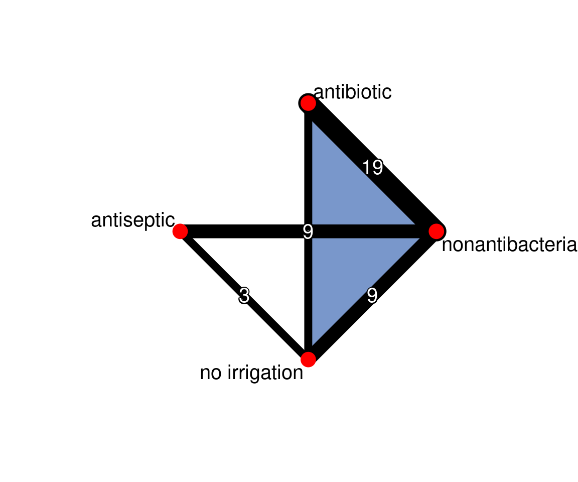
The probability that each treatment is ranked 1st (i.e. best) can be calculated using the netrank() function. These probabilities are called p-scores and they strongly favour antibiotic. A rankogram can also be generated using the rankgram() function and then plotting using plot(). Both the p-scores and rankograms agree with the ranking provided by multinma, but the probability of antibiotic being best is higher due to the lower estimated effect of antiseptic (the second best treatment) in the netmeta analysis. The probability of any treatment being best should be interepreted with caution as it can be unstable if uncertainty is high.
# P-score probabilities
netrank(icl_fit_re, small.values = "good")
P-score
antibiotic 0.9612
antiseptic 0.6705
no irrigation 0.1964
nonantibacterial 0.1719# Plot the rankograms
plot(rankogram(icl_fit_re, small.values = "good"))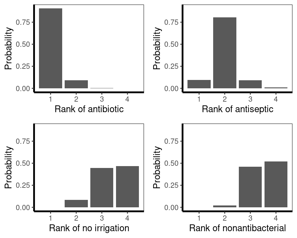
Finally, Surface Under Cumulative Ranking Area (SUCRA) scores, which are the sum of the area under the cumulative rankograms, can be estimated, with favoured treatments being closer to \(1.00\). These scores also favour antibiotics.
# Can also estimate SUCRA with sampling
netrank(icl_fit_re, small.values = "good", method = "SUCRA")
SUCRA
antibiotic 0.9687
antiseptic 0.6603
no irrigation 0.2090
nonantibacterial 0.1620
- based on 1000 simulationsInconsistency is assessed using the netheat() function (Jackson et al., 2012; Krahn et al., 2013). The underscores are used for comparisons in multi-arm trials. For example, "nonantibacterial:no irrigation_nonantibacterial:antibiotic:no irrigation" refers to the nonantibacterial vs. no irrigation comparison within the nonantibacterial vs. antibiotic vs. no irrigation studies.
The grey square size indicates the contribution of direct evidence in a column on the estimate in each row. For example, we see that direct nonantibacterial vs. antibiotic evidence (col 4) has a large impact on the estimate for no irrigation vs. antibiotic (row 3), among others.
The colours in the diagonal show the inconsistency contribution of each design. Dark-yellow/orange/red means greater contribution, and we see that nonantibacterial vs. no irrigation and nonantibacterial vs. antiseptic contribute somewhat more.
The off-diagonals show the change in inconsistency between direct and indirect evidence in the row after relaxing the consistency assumption for the effect of the design in the column. Blue colours increase consistency, yellow/orange colours decrease consistency. Blue therefore means the column-evidence supports the row-evidence, while dark yellow/orange means that the column evidence is inconsistent with the row-evidence.
netheat(icl_fit_re, nchar.trts = 7)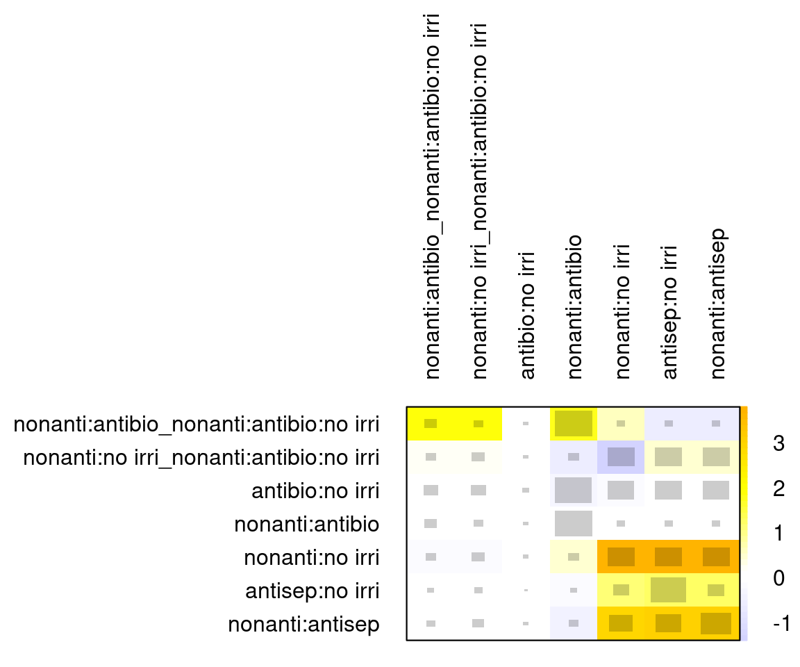
We see three comparisons for which detaching leads to a decrease in inconsistency (last three columns):
- antiseptic:no irrigation
- nonantibacterial:antiseptic
- nonantibacterial:no irrigation.
We can also compare this to the results of the decomp.design() function. The Q statistic P-values go up if any of these three is detached. So it seems these are the source of potential inconsistency, which aligns with the node splitting analysis conducted using multinma. Lastly, we also see that a \(Q\)-test of the inconsistency is not significant anymore once we allow for full design-by-treatment interactions in a random-effects model (\(Q\)=5.27, \(p\)=0.26). Note however that this fully specified model is meaningless for treatment effect estimates. It is useful to assess assumptions, but if it gives a substantially better fit it cannot be used to obtain estimates for inference. Instead it would be necessary to go back to the studies or get clinical input on why there is evidence of inconsistency.
# Compare to decomp.design results (esp. Between-designs Q section)
decomp.design(icl_fit_re)
Q statistics to assess homogeneity / consistency
Q df p-value
Total 71.14 38 0.0009
Within designs 60.70 34 0.0032
Between designs 10.44 4 0.0337
Design-specific decomposition of within-designs Q statistic
Design Q df p-value
nonantibacterial:antiseptic 22.38 8 0.0043
nonantibacterial:no irrigation 15.05 6 0.0198
nonantibacterial:antibiotic 22.77 16 0.1199
nonantibacterial:antibiotic:no irrigation 0.39 2 0.8220
antiseptic:no irrigation 0.11 2 0.9476
Between-designs Q statistic after detaching of single designs
(influential designs have p-value markedly different from 0.0337)
Detached design Q df p-value
antiseptic:no irrigation 2.50 3 0.4756
nonantibacterial:antiseptic 2.50 3 0.4756
nonantibacterial:no irrigation 3.47 3 0.3251
nonantibacterial:antibiotic 9.40 3 0.0244
nonantibacterial:antibiotic:no irrigation 8.19 2 0.0167
antibiotic:no irrigation 10.33 3 0.0160
Q statistic to assess consistency under the assumption of
a full design-by-treatment interaction random effects model
Q df p-value tau.within tau2.within
Between designs 5.27 4 0.2608 0.4459 0.198810.5 Discussion
In this chapter, we have given the necessary theory and code to run network meta-analyses in R. We began with a conceptual introduction to network meta-analysis through the consistency assumption, with illustration on binary outcomes. We explained both Bayesian and frequentist approaches for estimation and noted the subtle differences in interpretation of results depending on the method of estimation. We closed the conceptual introduction with model assessment, network meta-regression, and tests for inconsistency. These concepts were then put into practice on the SSI NMA and implemented in the Bayesian multinma and frequentist netmeta packages. In both packages we should the estimation of fixed and random effects NMA, estimation of relative effects, graphical summaries of results, rankograms, and tests for inconsistency. Using multinma we showed how to perform a meta-regression on contamination level while netmeta was used to visualise inconsistency contributions with the powerful netheat function. Results of both packages were aligned. With this chapter, a reader would be in a position to run a variety of relevant NMAs on new applications. However, there are some important topics that have not been presented.
Our application was to binary outcomes which we modelled with a binomial likelihood and logistic link function (Dias et al., 2018, 2013a). NMAs can be conducted on many different data types and alternative likelihoods and link functions have been extensively described in the literature, including in the multinma vignettes. Continuous outcomes, such as change in walking distance or biomarkers from baseline, could be modelled with a Normal likelihood and identity link. This can be implemented in multinma by specifying the y and se arguments for set_agd_arm(), which are mean and standard error of the outcome, instead of r and n. Count data with exposure times, such as the number of new cases of diabetes or occurrence of treatment related adverse events, can be modelled using a binomial likelihood and cloglog link function. This allows the inclusion of an offset for exposure time. This model is implemented in multinma with r and n as the data to pass to set_agd_arm(), and then by specifying the arguments link = "cloglog" and regression = ~offset(log(time)) in nma(). Another common data type are counts of outcomes across exclusive categories, such as 50%, 75%, or 90% reduction in symptoms on the Psoriasis Area and Severity Index (PASI) in plaque psoriasis (Phillippo et al., 2023). These could be modelled using an ordered multinomial likelihood and probit link function. This model is again implemented in multinma, this time with the multi() function to set up ordered categorical outcomes in set_agd_arm(). Our approach can also be extended to the case where Individual Patient Data (IPD) are available from all studies, rather than only aggregate data. IPD NMA has been implemented in multinma and is viewed as the gold standard for NMA as it can adjust for differences in baseline characteristics and features of trial design.
The above are relatively simple modifications: all fall within the generalised linear modelling approach to NMA we have described, and all can be implemented in multinma (Dias et al., 2013a). A range of techniques have been developed for NMA on survival outcomes, such as Overall Survival (OS) and Progression Free Survival (PFS) in oncology. These include models based on standard parametric models, fractional polynomials, piecewise constant assumptions, and Royston-Parmar splines (Cope et al., 2020; Freeman and Carpenter, 2017; Jansen, 2011; Lu et al., 2007). The advantage of these approaches over, for example, NMA on reported hazard ratios, is that they have the flexibility to allow for non-proportional hazards. These models, and their application to indirect treatment comparison, have been extensively compared in the literature and will be partly discussed in Chapter 7. These models highlight a limitation in our presentation of R for NMA as they have not been implemented in easy-to-use packages. Publications instead provide code in the Bayesian modelling languages BUGS, JAGS, and Stan, which must be linked to R using packages R2OpenBUGS, rjags or rstan, respectively (Carpenter et al., 2017; Lunn et al., 2013; Plummer et al., 2003; Team, 2023). However, recent updates to the multinma package added functionality for NMA of survival outcomes, implementing standard parametric models as well as piecewise exponential and flexible M-spline hazards models, all of which can be specified to allow for non-proportional hazards (Phillippo et al., 2024).
A further modification to NMA is to consider if there is imbalance in treatment effect modifiers across the contributing studies (Phillippo et al., 2018). If these are imbalanced and no adjustment is made, the NMA could give biased estimates. If there are effect modifiers, and regardless of whether the studies are balanced, the target population of the NMA would need to be specified as it would depend on included distribution of effect modifiers. Matching Adjusted Indirect Comparison (MAIC) and Simulated Treatment Comparison (STC) were early approaches to population adjusted indirect treatment comparison which balanced the IPD from one study to match its effect modifier distribution to that of an aggregate data comparator study (Caro and Ishak, 2010; Signorovitch et al., 2012). MAIC and STC were limited to pairwise comparisons and single studies on each contrast, and their target population had to be that of the aggregate data study. Multilevel Network Meta-Regression (ML-NMR) is a more general approach that overcomes these limitations and has been implemented in the multinma package (Phillippo et al., 2020). These methods, and ML-NMR in particular, are described in more detail in Chapter 13.
The final important topic we have not considered is how to handle scenarios where the evidence networks are disconnected (Stevens et al., 2018; Thom et al., 2022). The most commonly employed methods are unanchored forms of MAIC and STC, both of which have been implemented in R but required IPD from at least one study (Phillippo et al., 2016). A variety of approaches are available in cases where only aggregate data are available, including hierarchical models for merging related treatments, dose response models, multiple components analysis, matching of control arms, and prediction of response to a reference treatment (Leahy et al., 2019; Pedder et al., 2021; Rucker et al., 2021, 2020). Matching of control arms and predicting response to reference treatment have also been applied to the inclusion of single-arm studies in NMA (Leahy et al., 2019; Thom et al., 2022). Although initial publications of these methods for disconnected evidence may have relied on custom JAGS or BUGS code, these approaches are increasingly being implemented into R packages such as gemtc, multinma and MBNMAdose.