parameters <- list(
  # ~ Model settings ------------------------------------------------------
  settings = list(
    state_names = state_names,        #state names
    Dr_C = input$Dr_C,                #Discount rate: costs
    Dr_Ly = input$Dr_Ly,              #Discount rate: life years
    THorizon = input$THorizon,        #Time horizon
    state_BL_dist = c(1, 0, 0, 0),    #starting distribution of states
    combo_dur = 2                     #number of states with combination therapy
  ),

  # ~ Transition probability matrices (TPMs) ------------------------------
  transitions = list(
    TPM_mono = TPM$mono,   #Control arm transition probability matrix
    TPM_combo = TPM$combo  #Intervention arm transition probability matrix
    ),

  # ~ Costs ---------------------------------------------------------------
  Costs = list(
    DM_CC_costs = data.frame(
      unlist(DM_CC_costs$state_A),
      unlist(DM_CC_costs$state_B),
      unlist(DM_CC_costs$state_C),
      unlist(DM_CC_costs$state_D)
    ),
    drug_costs  = drug_costs,
    state_costs = state_costs
  )
)14 R and shiny in HTA
Rose Hart
Lumanity, Sheffield, UK
Darren Burns
Delta Hat, Nottingham, UK
Mark Strong
University of Sheffield, UK
Andrea Berardi
PRECISIONheor, UK
Dawn Lee
University of Exeter, UK
14.1 Introduction to the shiny package
14.1.1 What is shiny and how can it help me make my models accessible?
shiny is an R package that makes it easy to build interactive web applications within R (Chang et al., 2021). shiny provides a wrapper around your existing functional R code, allowing you to host stand-alone applications on a web page, embed them in rmarkdown or quarto documents and build dashboards. This is helpful if the model target audience is unfamiliar with R, as the application can be used entirely within a web browser and without the user being exposed to any R code (or even having R installed on their local machine!). The functionality available within the shiny package alone is considerable, and the package undergoes regular updates. CSS themes, html, and JavaScript can also be used to further develop the graphics and interactive capabilities of your shiny application.
The optimal modeling platform is one that is fast, transparent, and flexible to required changes in modeling assumptions or supporting data sets, while remaining user friendly (Hart et al., 2020). R alone fulfills the majority of these requirements. However, as a script-based language, R can seem daunting to newer users. shiny is increasingly used by health economic modelers as it allows the developer to make economic models accessible to all types of user (Chang et al., 2021).
A model built with shiny comprises two parts: a user interface (ui) and a server. The ui forms the basis of how the user interacts with the model and is designed to be user friendly. The server operates as the engine.
A shiny application allows the user to amend inputs in a similar manner to Excel, without needing to access the background R code. In this sense, an R-based model using shiny is comparable to an Excel-based model developed in part using Visual Basic for Applications (VBA) code, but with the capacity for complex statistical analysis, model flexibility and high-quality visuals.
Of course, a shiny interface is not sufficient for a reviewer to understand the underlying mechanisms of a model. Nevertheless, the use of shiny can serve as a bridge between complex functionality and model accessibility, making it easier to directly communicate the results of a model to decisions makers and other stakeholders. (Smith and Schneider, 2020)
14.1.2 What types of models could I use shiny for?
This section describes four types of economic model for which a shiny interface could be used to aid accessibility. These have been chosen to illustrate the advantages of being able to consolidate and calculate in real time the underlying statistics informing health economic decision problems, and of providing the user with an intuitive means of interacting with the data – features that have the potential to improve both the quality of decision making within the pharmacoeconomic space and the efficiency with which decisions are made. There are, of course, plenty of other types of model where this is the case.
We provide basic information on the build process and requirements of these economic models. Some of the examples noted here will be expanded on later within this chapter. It is clear to see that use of R in combination with shiny has the potential to provide significant benefits in health economics and outcomes research (HEOR).
Early modelling and feasibility assessment
Model objective
- Assess feasibility of HTA success
- Understand economically justifiable price
- Identify data gaps and key uncertainties
How can R/shiny help?
- Increase scalability and consistency
- Incorporation of multiple indications and countries
- Integrated end-to-end analysis means fast updates to the model as soon as trial data become available
- Reduce errors and increase efficiency
- No copy-and-pasting
- Export outcomes to
PDF,Word, andPowerPoint - Version control capabilities using
Gitallowing parallel working and tracked changes - User-friendly front-end
- Improved graphics for presentation
HTA models
Model objective
- Demonstrate the economic value of a product to HTA decision makers
How can R/shiny help?
- Increase scalability, flexibility, and consistency
- Incorporation of multiple indications, data cuts, countries, and modelling strategies
- Reduce errors and increase efficiency
- No copy-and-pasting
- Export outcomes to PDF, Word, and PowerPoint
- Version control capabilities using
Gitallowing parallel working and tracked changes - Increase speed: probabilistic sensitivity analysis and one-way sensitivity analysis are approximately nine times faster (Hart et al., 2020)
Examples
intRface™(Hart et al., 2020)- IVI open-source value tools (Jansen et al., 2019)
- Four-state Markov tutorial (Smith and Schneider, 2020)
Eliciting inputs/informing parameters
Model objective
- Conduct and present analyses
- Allow experts to provide informed judgments
How can R/shiny help?
- Increase scalability and flexibility
- Incorporation of multiple data sets and analysis strategies
- View the end outputs of analyses live during expert engagement
- Reduce errors and increase efficiency
- A continuous, end-to-end process is possible, from input of results or analyses through to collation and reporting
Examples
BCEAweb(Baio et al., 2017)SAVI(Strong et al., 2014a)PriMERSHELF(Strong et al., 2014b)- FDA drug safety reporting ratios (
https://openfda.shinyapps.io/RR_D)
Direct-to-payer/value tools
Model objective
- Demonstrate the economic value of a product direct to payers
How can R/shiny help?
- Increase scalability and consistency
- Incorporation of multiple indications and countries
- Improved graphics for presentation
- View the end outputs of analyses live during payer engagement
- Automatically export outcomes to generate payer leave pieces
- Ability to make available online as an open-source model for payers to use
Examples
- IVI open-source value tools (Jansen et al., 2019)
- Immunology treatment sequence value tool (Hart et al., 2024)
14.1.3 How can I learn more?
A tutorial covering the basics of how to build an application using shiny is available from the Rstudio website (Chang et al., 2021). It includes a set of exercises and takes approximately half a day to complete. We would recommend investing the time to go through this tutorial before attempting to add a user interface to an R-based economic model.
The next sections provide:
- Section 14.2: Additional detail regarding examples of shiny applications in health economics
- Section 14.4: Guidance on the practicalities of building a shiny application including
- Health technology assessment (HTA) requirements
- Coding for transparency
- Quality control (QC)
- Deployment
- Workflow and version control
In addition, the online version of this book (available at the website https://gianluca.statistica.it/books/online/rhta) also provides a step-by-step guide to building an application using shiny to wrap around a HTA model.
14.2 Examples of shiny applications in health economics
The Rstudio Shiny gallery provides many examples of different shiny applications, which can be used for inspiration. There are also numerous examples of shiny applications within HEOR. Table 14.1 provides a non-exhaustive list of publicly available HEOR applications built using shiny. Each of these applications serves the purpose of adding an interface onto a process that was written in R, thereby improving accessibility to non-R users and enabling online publication for worldwide distribution. Most the applications described in Table 14.1 and in the Rstudio gallery are hosted using the shinyapps.io website, which links with the Rstudio environment of the programmer and allows easy publication of applications online.
R with shiny could be advantageous
| Application | Authors / group | Model access and summary |
|---|---|---|
intRface™ |
BresMed Health Solutions Ltd (Hart et al., 2020) | This model (https://shorturl.at/apzK6) is part of an explicit comparison between shiny and Excel for modeling a hypothetical decision problem of a non-specified CAR T-cell therapy in B-cell acute lymphoblastic leukaemia (Hart et al., 2020) The purpose of this model is to showcase the potential of using shiny applications for complex modelling, and includes analyses such as propensity score matching and mixture cure modelling alongside standard partitioned survival (Chapter 7) and state transition modelling approaches (Chapter 11). |
IVI |
Innovation and Value Initiative (IVI, Jansen et al., 2019) | IVI has built three models using shiny; the first is for rheumatoid arthritis (https://shorturl.at/cvxS6), the second is for non-small cell lung carcinoma (https://shorturl.at/bdtKO) and the third is for major depressive disorderusing publicly available efficacy data (https://shorturl.at/qwzC5). |
Tutorial using the Sick-Sicker model |
Smith and Schneider (2020) | This application provides an extensive tutorial for the application of a shiny front-end to the Sick-Sicker model developed by DARTH (https://shorturl.at/cuzL8) |
QALY shortfall calculator |
University of Sheffield, University of York and Lumanity (McNamara et al., 2023) | This application is referenced in NICE (2022) and can be used to calculate quality adjusted life expectancy and proportional and absolute shortfall in order to calculate whether or not severity modifers are relevant (https://shiny.york.ac.uk/shortfall) |
SAVI |
University of Sheffield School of Health and Related Research (Strong et al., 2015) | The Sheffield Accelerated Value of Information (SAVI; http://savi.shef.ac.uk/SAVI) model takes probabilistic sensitivity analysis from the user and allows the user to generate i) standardized assessment of uncertainty; ii) overall EVPI per patient, per jurisdiction per year and over the decision relevance horizon; and iii) EVPPI for single and groups of parameters (see Section 1.8). |
BCEAweb |
University College London (Baio et al., 2017) | Part of the BCEA package. On loading the package, it can be accessed by running BCEAweb() and it will deploy locally. Provides an interface to the BCEA package, which is designed to produce health economic evaluations using user-inputted results from a large number of model simulations for all the relevant model parameters. The model uses this input to present the economic and uncertainty analysis results alongside a value of information analysis (Section 1.8). Can be accessed also at https://egon.stats.ucl.ac.uk/projects/BCEAweb |
GH CEA Registry |
Center for Evaluation of Value and Risk in Health (2019) | The Global Health Cost-Effectiveness Analysis (GH CEA) Registry is a database that compiles articles utilizing the cost per disability-adjusted life year metric to measure the efficacy of health interventions. The database is presented in a shiny application (http://ghcearegistry.org/ghcearegistry) |
PriMER |
University of Washington (The Comparative Health Outcomes Policy and Economics Institute, CHOICE, 2020) | The PriMER tool predicts the diffusion of personalized medicine technologies, accounting for the disease, associated test and population. The included calculations are based on a series of preference studies conducted with patients, providers and healthcare payers (https://uwchoice.shinyapps.io/primer) |
14.3 Building a shiny application
14.3.1 Components of a shiny application
As introduced above, applications built using shiny usually consist of two R objects: ui and server. The R command shinyApp() requires both a ui object and a server object in order to generate the application (RStudio, 2017). The alternative command, runApp(), can be used if the scripts generating the ui and server objects are separate, as we would recommend (RunshinyAppRStudio?).
The user interface (ui) list
The ui list contains instructions for the layout of the application, as well as interactive components.ui objects are very flexible; they are suitable for simple presentations of calculations and results as well as complicated interactive inter-dependencies. Due to the web design basis of the shiny functions, the look and feel of the ui can be manipulated using HTML and CSS, as with any standard web page.
The shiny application structure allows several different approaches to programming the ui. For instance, the ui can be broken down into several different files to avoid lengthy blocks of code. Alternatively, ui elements can be generated inside of the server scripts, which allows additional flexibility or interactivity.
The server list
A server object is defined as an R function. This R function usually has three arguments:
inputoutputsession
input and output are lists. The input list contains the input information from the UI at any given time, while output contains the outputs being sent back into the UI after any calculations have taken place. Both the input and output lists exist at the same time and are also interdependent. This means that while a shiny application is running, a constant feedback loop is in place; the server reacts to the individual arguments in the input list by executing functions that are related to any of the inputs when they are detected to have changed. This process then creates outputs that return to the UI. This is closely analogous to a Microsoft Excel workbook when calculations are set to ‘Automatic’.
As computational feedback loops can easily occur in this context, there are several mechanisms available to monitor and manage computation in shiny applications. Within shiny, this is referred to as reactivity. There are many functions that can be used to control the reactivity in the model. For example:
reactive(): Arguments that are wrapped inside of areactive()function will recalculate given any stimulus, i.e. any change in inputseventReactive(): These arguments will recalculate only upon an event, which is specified by the programmer (e.g. pressing a button or switch)
There are many other functions that control what happens when in a model aside from the two that are given as examples here, each with a particular purpose and level of reactivity to the shiny application environment. This facilitates flexibility and control when designing an application.
Overall, the flexibility of a shiny application is the same as the flexibility of general R code. However, because model functions are wrapped within shiny functions, there are some differences in the syntax and flow of computations when compared to basic R scripts. There are online courses that introduce different shiny-specific concepts, while also explaining how to write these functions, and it would help to be familiar with these and use them in conjunction with this section (Shinytutorial?) (DataCamp, 2020). The RStudio tutorial is a good place to learn the basics of working with shiny.
The sub-sections below outline the step-by-step process of building a shiny application. The examples used are freely available in a public GitHub repository, providing full-code examples of the techniques outlined in each sub-section. The steps below can also be used independently of the code examples as a more general guide to the methods and functions used in building a shiny application.
14.3.2 Components of a shiny application
For health economic modelling using R, we recommend developing a basic working model in R before involving shiny. This is for a number of reasons. Firstly, from our experience of developing such applications, the process of quality control (QC) checking and debugging becomes more difficult once the set of R scripts comprising the health economic model have been wrapped in shiny functions application. Secondly, during the development of the health economic model, ideas will typically be generated determining exploration of first order, second order, and structural uncertainties. These will often influence the approach to facilitating and incorporating appropriate analyses, which is easier to implement when the scripts are not already contained within server or ui objects. Thirdly, when designing the ui for a shiny application, the programmer must decide on the level of information available to the end user of the application. For instance, Excel is seen to be transparent due to its high level of perceived verbosity – a user can see all the calculations in the model simply by clicking on the cells. Once a model is functioning, and it is understood which calculations should be presented, an informed decision on how to present the intermediate calculations can be made. Finally, in health economics, code-based models have a reputation of lacking transparency, with the term ‘black box’ being commonplace. However, a well-designed shiny application presenting all relevant information, QC checks, intermediate calculation steps and outputs can achieve a high level of transparency. Writing the initial core of the model in a neat, annotated, and transparent way is more easily achieved without shiny. The programmer can then subsequently focus on achieving the same level of transparency within the shiny framework.
There are many packages that assist with producing aesthetically pleasing outputs that can be highly informative to the user and aid transparency within an R code, which can then be directly used into the ui as an output item. For example, the DT package produces neat tables that are easily customized. Some features include static columns, scrolling, search boxes, paging, and ordering by clicking on columns. DT tables can be used to present data independently of shiny applications, allowing the programmer to visualize the outputs of the code before then adding to the ui (Xie et al., 2021).
ggplot2 is another fundamental package for displaying model outcomes visually. This package can produce a wide variety of appealing and informative graphs that can be used by the programmer at the design stage of the application before wrapping in shiny functions. It is also worth noting that the ggplot2 functions can be used with user-amendable switches (e.g. to toggle a data overlay), sliding scales (e.g. amendable axes limits), and a floating window that provides x and y coordinates (the latter being a feature of shiny itself) to create dynamic and interactive plots. Before including these features, we recommend considering the level of interactivity needed in the application when deciding on the desired graphical output (Wickham, 2016) (RStudio, 2020a).
While the incorporation of shiny after development of the core scripts may lead to changes in functionality and calculations, we recommend keeping the original separate model script up to date. This allows for:
- Easier late-stage QC checking
- Cross-checking the
Rscript with theshinyapplication to ensure they produce the same results.
The second point is very important if the shiny application includes multiple layers of reactivity, as it will help the programmer ensure that the correct processes are happening in the correct order and are triggered when the user expects.
NoteCode Example 1
An example of a model within an R script without shiny is shown in the ‘1. R code for HIV model (no shiny).R’ file. This script replicates the HIV/AIDS model from Section 2.5 in Briggs et al.(Briggs et al., 2006) Please take the time to go through and broadly understand this code before moving onto the next example, as this code is adapted throughout all the subsequent code examples. The code is organized with all of the user-defined functions stated and commented at the top of the code, before splitting the model code up into sections. Because R code is linear, this can make it very easy to perform QC checks and trace through.
Users running this code will see that the R script includes data tables and graphs to inform the outputs and also QC messaging. The intermediate calculations and results were written so that they can be directly wrapped by shiny functions; any result that is used as an input to another function, or is to be displayed in a graph or table, is returned to the top level. Additionally, the input object is produced as a list, which allows the programmer to identify the inputs that they may want to have as user amendable in the front-end of the code.
When designing models, it is a good idea to ensure that there is a central list where inputs can be gathered and then used as a single list to inform all of the functions and the production of the results in the model. This has been done in this example in the parameters list. Arranging inputs in this way is especially important in a shiny application because, like an Excel model, there is the option for the model to instantaneously update and be reactive. Setting these reactive dependencies is an important part of designing a shiny application, so having a central list to allow a break to control the level of reactivity is recommended. This will be explored in Code Example 3 onward.
The script below shows the parameters list within the model code. This indexes all inputs into sub-lists and all information that the model is dependent on is passed through this list to the model engine functions.
14.3.3 Designing the user interface
The UI is the part of the application that faces the user. The ui object is the layout of the inputs and outputs in the application, as well as any additional text to be included in the web page. One of the packages that assists programmers with layout design is shinydashboard.(Chang and Borges Ribeiro, 2018) This package allows programmers to produce and customize an application header with a navigation bar to specified tabs.
The design of the UI can also be directed using CSS. We recommend looking at the examples (RStudio Shiny gallery(RStudio, 2020a)) and experimenting with customization (shinydashboard – Appearance page(RStudioshinydashboard, 2020)) to develop a UI design before programming the application. As CSS and HTML are the standard languages of internet web pages, there are a vast number of resources available on the customization of layout, themes, and aesthetics.
Once the look and feel of the ui has been determined, then the layout of the application is a sensible next step. As with Excel, when formulating the layout and types of information presented within the application, the audience must be considered. There may be multiple audiences with different needs – such as company stakeholders, evidence review groups or HTA reviewers, and local payers – wishing to interact with your application, and you will need to consider all of these. Once a desirable layout has been implemented, it is important to consider the options being provided to the user and their compatibility with the server.
An additional consideration when designing the ui script is how the user or developer of the application will be able to perform a QC check on its functionality. Examples of this include ensuring that there are numerous intermediate calculations presented so the user can see how the values flow through the model, and presenting tables with the results of appropriate application tests. We advise using the rmarkdown package to generate reproducible reports of the model functionality, QC checks, and results.(Allaire et al., 2021) (Allaire et al., 2021) (Allaire et al., 2021) rmarkdown can be used from within a shiny server, meaning that such reports can be created by the user with a simple button press within the UI.
Code Example 2
An example of a model UI within a shiny application is in the ‘2. Shiny UI layout.R’ file. This application uses shinydashboard functions to create a simple model layout with a header bar and navigation panel. The navigation panel is ordered according to the different inputs, information and outputs in the model, with icons added to represent each tab.(RStudio, 2020b) The control widgets that make up the inputs are inside boxes that are coloured according to status.(RStudio, 2020c) The overall design of the page is influenced by the shinydashboard appearance guidance for a clear but versatile look.(Chang and Borges Ribeiro, 2018)
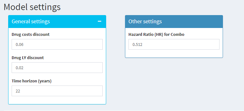
Tables of the input clinical data and state and drugs costs are presented in the tabs using the functions from the DT package.(Xie et al., 2021) Placeholders have been added by text to plan the layout of results tables and graphs. The ‘Test outputs’ box is for the user to view the active values in the server; this way the user can see that the interaction with the selected inputs (in this case the Time horizon and the Combo arm hazard ratio) is read by the server, which in turn is rendered as a text output. This is in preparation for future code versions, where the inputs are read by the server and then passed through to the required functions.
Looking at the code itself, the ui and server are both presented in the app.R file. The shinydashboard functions dashboardPage, dashboardSidebar and dashboardBody are appropriately spaced and commented, allowing easy viewing for the programmer and reviewer. A similar approach is used for defining the input and output lists in the ui and rendering the outputs in the server function. Sections are used in the code to aid navigation.
Although this application is simple and does not have any functionality in the server (aside from presenting tables) the code is over 400 lines. Because the application code is read as two large functions, as opposed to multiple small functions in Code Example 1, navigation and commenting are all the more important in shiny applications because it is not possible to run the individual code increments. Therefore, it is recommended that good sectioning and commenting code be used throughout the application to assist both the developer and reviewer.
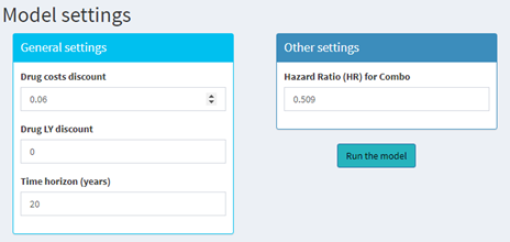
The following code is an example of how the ui code can be presented; it creates the two input boxes within ‘Model settings’ tab. The code is followed by the output viewed in the model UI.
dashboardBody(
  tabItems(
    tabItem(
      # ~~ Model settings --------------------------------------------------------
      tabName = "tab_Settings",
      tags$h2("Model settings"),
      fluidRow(          # `R` Shiny normally renders vertically. fluidrow allows horizontal layering
        column(          # Columns within fluidrow. the width of the whole page is always 12
          4,
          box(
            title = "General settings",
            width = 12,                  # This '12' refers to the whole space within the column
            solidHeader = TRUE,          # Whether you want a solid colour border
            collapsible = TRUE,          # Collapsible box
            status = "info",             # This is the reference to the colour of the box
            numericInput(
              inputId = "Dr_C",
              label = "Drug costs discount",
              value = 0.06,
              max = 1,
              min = 0,
              step = 0.01
            ),
            numericInput(
              inputId = "Dr_Ly",
              label = "Drug LY discount",
              value = 0,
              max = 1,
              min = 0,
              step = 0.01
            ),
            numericInput(
              inputId = "THorizon",
              label = "Time horizon (years)",
              value = 20,
              max = 100,
              min = 10,
              step = 1
            )
          )
        ),
        column(
          4,
          box(
            title = "Other settings",
            width = 12,
            solidHeader = TRUE,
            collapsible = FALSE,
            status = "primary",
            numericInput(
              inputId = "combo_HR",
              label = "Hazard Ratio (HR) for Combo",
              value = 0.509,
              max = 2,
              min = 0.001,
              step = 0.001
            )
          )
        ),

        ## Code continues
Code output viewed in UI:
14.3.4 observe and reactive
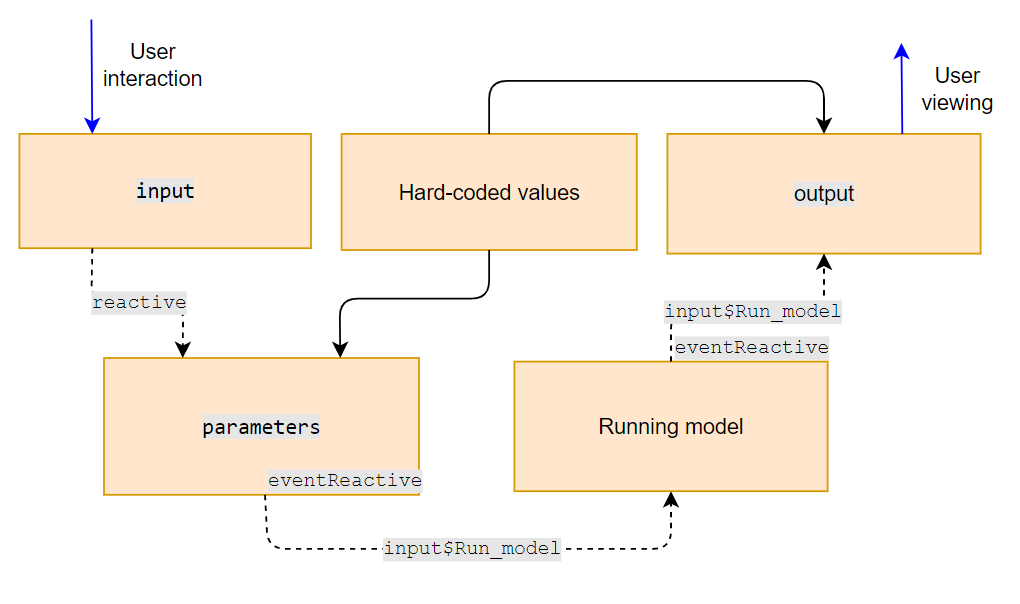
shiny server objects require the input list object. As shown in Figure @ref(fig:shiny-model-struc)), the object input originates from the ui object, which feeds into the input argument of the server function. The information from input list is then fed into the functions contained within server. Once those calculations are complete, the server populates the output list, which then feeds back into the ui object to be displayed. This process occurs continuously while a shiny application is active. As described earlier, the recalculation of objects within the server is referred to within shiny as reactivity. An object that reacts (i.e. recalculates in response) to external stimuli is referred to as a reactive object.
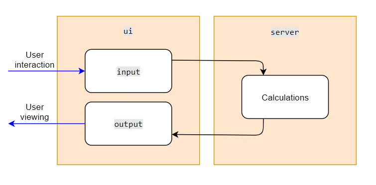
shiny application structureThe two simplest reactive objects are observe and reactive. observe and reactive are triggered for recalculation whenever there is any change whatsoever in the object inputs, each with a different purpose. observe executes a set of actions, whereas reactive produces an object. The difference between the two is illustrated in Figure @ref(fig:shiny-model-obsreac)).
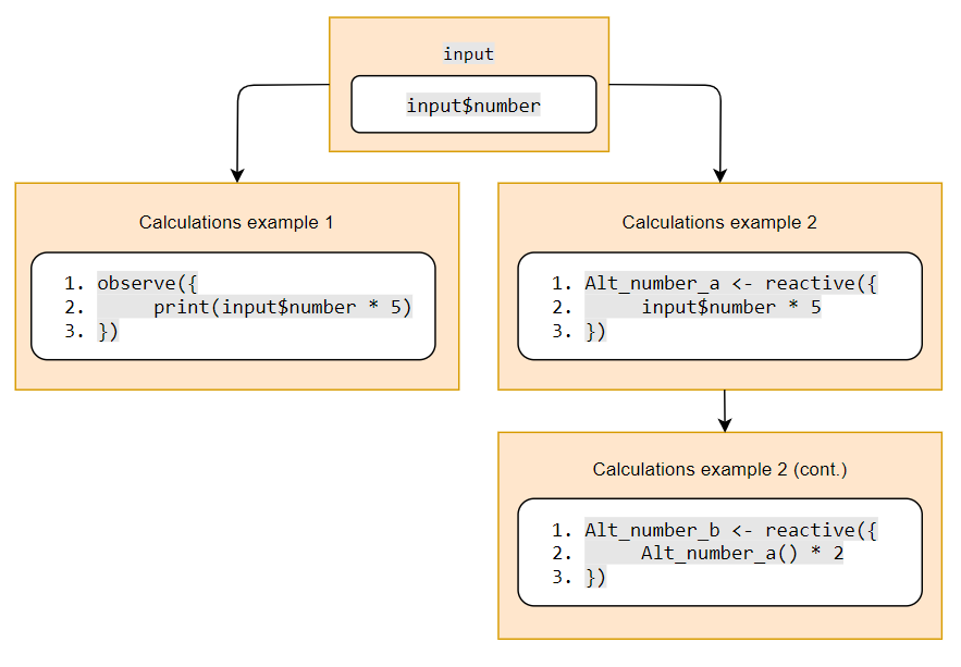
observe and reactiveIn this example, input$number is used by observe to multiply the input number by 5. It does not create an object, and in order to see the results in the R console, print must be used. Whereas, reactive is used to generate an object Alt_number_a, which can then be used in further calculations. In this example, Alt_number_a is included in another reactive calculation, creating the object Alt_number_b.
When writing the set of calculations to be performed in a shiny health economic model, we advise that this process is broken down into a chain of manageable chunks, rather than a few monolithic reactive calculations. This is because observe can be used to print some intermediate calculation results to the console, whereas no reliable QC process can be applied to large blocks of code which cannot be interacted with. We also recommend using reactive to generate objects for the output list during the process, as these can easily be incorporated into the UI to improve transparency and ease or reduce the QC process. An additional benefit of splitting up code and presenting numerous intermediate steps is that the reactivity of the model (i.e. how much and to what extent the model is recalculating) can be more easily monitored to maintain the responsiveness and efficiency of the calculations.
In the case of Figure @ref(fig:shiny-model-obsreac), every time input$number is changed in the script, the observe and reactive approaches will both recalculate. input$number * 5 will be calculated in both expressions, the results will be printed to the console in the case of the observe statement, and the objects Alt_number_a and Alt_number_b will be generated from reactive.
On the ui side, if an output containing the value Alt_number_a() is created, this will change too if input$number is changed. Limiting the level of reactivity is an important consideration for keeping the model run times low and to control when particular functions are executed, and we address how to deal with this issue in the next section.
Both observe and reactive are useful for performing model calculations while designing the model functionality to link the input and output objects. Provided that the design stage has been thorough, there should be minimal difference between the design code and the application code, except for the shiny wrapping functions and the separation into ui and server objects.
Code Example 3
This code brings together the functionality design from Code Example 1 and the ui design in Code Example 2. This code uses the observe and reactive functions to link together the input list from the ui to the functions in the server to produce the output list. Producing the model graphs and tables in Code Example 1 improves the efficiency of this process; you will notice as you go through the Code Example 3 that there are significant similarities to the layout and structure of Code Example 1.
This application is also laid out in three separate scripts: app.R, server.R and ui.R. This naming format allows the scripts to be identified by R as an application, and allows the runApp() function to be used along with its associated arguments for activating the app.
This code is in the ‘3. Shiny app with observe() and reactive()’ file. It uses two different types of intermediate calculation reporting to demonstrate how each can be used: printing to the UI, and printing to the console. Experimenting with changing the input values in the ui and observing the reaction within the ui text outputs and console messages will allow the user to view the active values in the server and the reactivity of the model.
Because of the length of the code, segments are presented in the examples below. The settings inputs are not changed from Code Example 2, but are now found within the ui.R script. Drug unit costs are not changed from Code Example 2, but are now rendered within the server.R script. drug_costs is now wrapped in reactive() as it is an object that is dependent on input$THorizon and needs to be subsequently used in downstream objects and functions, such as the parameters list.
   drug_costs <- reactive({
    list(
      AZT_mono = rep(Drug_unit_costs$AZT_mono,input$THorizon),
      lamivudine = c(rep(Drug_unit_costs$lamivudine,2),rep(0,input$THorizon - 2)),
      combo = rep(Drug_unit_costs$AZT_mono,input$THorizon) +                                                            c(rep(Drug_unit_costs$lamivudine,2),rep(0,input$THorizon - 2))
    )
  })
The parameters list is also wrapped in reactive() as it is dependent on other reactive objects and input list objects. It is also used to display in tables and in the functions to run the model. Note that drug_costs is referenced as a function in this code because it is now a reactive object.
parameters <- reactive({
    list(
      # ~~ Model settings --------------------------------------------------------
      #These are laid out as an embedded list to show off what you can do with a list
      settings = list(
        #state names
        state_names = state_names,
        #Discount rate: costs
        Dr_C = input$Dr_C,
        #Discount rate: life years
        Dr_Ly = input$Dr_Ly,
        #Time horizon
        THorizon = input$THorizon,
        #starting distribution of states
        state_BL_dist = c(1, 0, 0, 0)
      ),
# ~ Transition probability matrices (TPMs) ----------------
…, Transition probability matrices not presented for this illustrative example
# ~ Costs --------------------------
      Costs = list(
        DM_CC_costs = data.frame(
          unlist(DM_CC_costs$state_A),
          unlist(DM_CC_costs$state_B),
          unlist(DM_CC_costs$state_C),
          unlist(DM_CC_costs$state_D)
        ),
        drug_costs  = drug_costs(),
        state_costs = state_costs()
      ))
  })
14.3.5 observeEvent and eventReactive
observeEvent and eventReactive are similar to observe and reactive, except that instead of reacting to any change in the input list, they are only reactive to specific inputs at the discretion of the programmer. This way, the reactivity of the model can be controlled, and calculations only performed when required. Event-based reactivity is analogous to VBA macros within Excel-based health economic models, being triggered by actions like buttons, switches, or drop-down menu list selections. Like such VBA macros, it is important that the reactivity is intuitive to the user and that the user is informed of the flow of information throughout the process. Again, it is important to consider the appropriate use of reactivity, as this can provide some control of calculation flow and considerably affect the computational performance of the model:
-
Functionality – If there are numerous interrelated steps depending upon a single event (e.g. a button pressed to recalculate the cost-effectiveness model), then there is likely to be a desired order of calculations. Skipping steps in this ordering could mean that non-existent or superseded values are used in calculations without any visibility to the user. In cost-effectiveness modelling, we recommend using
eventReactiveobjects so that the programmer has full control over the order in which the model computes -
Speed – Too much reactivity can considerably slow down a cost-effectiveness model, due to the number of unnecessary computations. However, if there is too little reactivity (e.g. the user having to sequentially push a series of buttons to perform a calculation correctly), then the model can be confusing or even unusable, especially if the dependencies are obscure and the model is not laid out intuitively
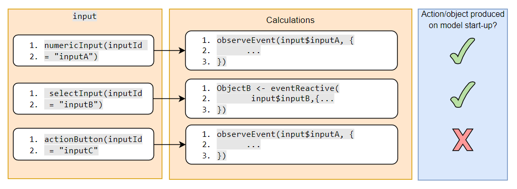
One technique to improve the process of writing shiny applications and controlling reactivity is knowing the point at which reactive objects are created. This is particularly important during model start-up, where non-existent or superseded objects can easily feed into a calculation and cause an error. Figure @ref(fig:shiny-model-strtup) illustrates this problem. In this model, there are three inputs defined in the input list in the ui: a numericInput, a selectInput and an actionButton. There are also two observeEvent objects in the server calculations, each printing a message. When the model starts, the message associated with the observeEvent dependent on the numericInput will appear in the console, but the observeEvent dependent on the actionButton will not. Events dependent on an actionButton, either using observeEvent or eventReactive, are not available on start-up, but most other input types such as numericInput and selectInput are. Therefore, in a model where there are numerous reactive elements dependent on a numericInput, these will exist without producing errors. However, if the input to a function depends on an input that is not available on start-up, such as one produced by an actionButton, then these calculations will either not execute at all, or they will execute in ways not intended by the programmer. It is therefore important during development to test the reactivity by printing to console and to the ui, to ensure that the required values exist and are reactive in the way that is expected. There are methods to control how the values go through the model and activate when planned, and these are explained in the next section.
One way for the programmer to plan out reactivity of their model – and to be able to effectively communicate reactivity to users and reviewers – is to produce a flow diagram, such as the one presented in Figure @ref(fig:shiny-model-reacflow). In this example, the input objects are interacted with by the user, and these feed via reactive (indicated by the dashed line) into the parameters object. Hard-coded values are also used in the parameters object and are presented in tables in the output list for the user to view, but these elements are not reactive (as indicated by the solid lines). The parameters list is then fed into functions that run the model and produce objects in the output list, but steps concerning the running of the model and the subsequent generation of results in the output list is controlled by eventReactive, and is dependent upon the user interaction with input$Run_model. Diagrams of the reactive pathways and dependencies within an application can be presented within applications as images, or exported from applications as part of a user guide.
Code Example 4
In this example, the model uses observe and reactive until the point of the parameters, then uses observeEvent and eventReactive after the parameters. The observeEvent and eventReactive objects are dependent on a button called input$Run_model. In this setup, the inputs are always reactive but are not used to run the model until input$Run_model is activated. In opening the application and interacting with the inputs, users will notice that the parameters sheet is populated with the live values, and the console prints the parameters whenever the inputs are interacted with. However, the results do not render until the ‘Run the model’ button is selected.
Because of the length of the code, segments are presented in the examples below. The setting inputs are not changed from Code Example 3, with the exception that they have an action button added under input$combo_HR, called input$Run_model
dashboardBody(
    tabItems( #This included the list of all the tabs
      tabItem( #This is where a single tab is defined (model settings)
        # ~~ Model settings --------------------------------------------------------
        tabName = "tab_Settings", # Tab ID
        tags$h2("Model settings"),
        fluidRow(    # fluidrow allows horizontal layering
…, General settings box not presented for this illustrative example
          column(
            4,
            box(
              title = "Other settings",
              width = 12,
              solidHeader = TRUE,
              collapsible = FALSE,
              status = "primary",
              numericInput(
                inputId = "combo_HR",
                label = "Hazard Ratio (HR) for Combo",
                value = 0.509,
                max = 2,
                min = 0.001,
                step = 0.001
              )
            ),
            column(        # Not all outputs need to be in boxes
              8,
              offset = 3,
              actionButton(inputId = "Run_model", label = "Run the model", style = "color: #000000; background-color: #26b3bd; border-color: #2e6da4")
            )
          ),
… Test outputs not presented for this illustrative example
      ))
Rendered output:
This model version uses reactive until the parameters list is created; because of this, the drug cost calculations and the parameters list are produced using in the same way as was shown in Code Example 3. The parameters list is then used only when input$Run_model is selected. An example of this is when the patient flow values are created; patient_flow is created as a list, patient_flow$disc is created as a sub-list to identify the discounting values to be used. patient_flow$disc$cost uses the time horizon and the annual discount from the parameters sheet to calculate the vector of discounting used at each cycle; it is only created when the input$Run_model button is activated.
patient_flow$disc$cost <- eventReactive(input$Run_model, {
    sapply(1:parameters()$settings$THorizon, function(n)
           {1 / ((1 + parameters()$settings$Dr_C) ^ n)})
  })
14.3.6 rhandsontable and conditionalPanel
There are many functions that can be used to enhance shiny applications, both within shiny and in other packages. Two of these functions are conditionalPanel and rhandsontable. Code Example 5 focuses on the use of these.
conditionalPanel is a simple way within shiny to make ui sections appear and disappear according to the settings of a particular object in the input list. This is useful if there are certain settings or pages that are only applicable when a particular setting is active.
The limitation of typical shiny inputs is that they are mostly only appropriate for inputting single values or settings. The functions within the rhandsontable package allow a table to be used as an input, similarly to Excel. rhandsontable is a JavaScript function adapted for use in R, so it can be flexible to changes including colour, number formats and also validation (restrictions to values, conditional formatting, etc.). It is also possible to add radio buttons, drop-down menus, heatmaps and rendering results; examples of this are available online. (Owen, 2022) Using rhandsontable is a good way of creating an Excel-like feel while also allowing much of the input data to be contained within one input. rhandsontable objects when used as inputs can trigger event-dependent reactive objects, meaning that changing one value in a table can trigger the associated chain of recalculations (just like in Excel).
Because rhandsontable objects exist both in the input list and the output list at the same time, they require some special treatment. rhandsontable objects are defined as outputs in server, rather than as inputs in ui (Figure @ref(fig:shiny-model-rhandsreacflow)). Inputs defined in the ui are available upon model start-up and can be used immediately in functions. However, inputs defined as outputs in the server are not available upon model start-up, and do not automatically ‘exist’ until the page and tab with the output object – in this case, the rhandsontable – is rendered. This is a problem, because reactive functions run on start-up; therefore, if a rhandsontable object is used as an input to inform a reactive or observe function, there will be errors when the model starts as the rhandsontable input will not exist at the time of first execution of the reactive or observe functions. There are a few things that can be done to solve this:
-
shinyhas a functionreq, short for ‘require’, which prevents computation of areactiveorobserveobject until after the arguments withinreqexist. For instance,req(input$number)within anobservewill never compute until the objectinput$numberexists, after which it will act as normal. This command is invaluable in preventing shiny applications from breaking when trying to compute using non-existent objects, as it will prevent the application from computing the value until the input exists. -
Alternatively,
is.nullcan also be used to test whether the input exists. If it does, then the input can be used, and if not, then the base case data informing the input can be used. Usingis.nullis recommended where the input is used to create multiple downstream processes that are required when the model starts up. In this instance, delaying the computation of the function relying on the input using req would not be appropriate as the object created by the input would then not exist, causing error in chain of functionality. -
If using
reactive, this can be changed toeventReactiveand made to be dependent on a button that would only be selected after the input exists. If this option is preferred but needs to be used on model start-up, then theclickfunction can be used to activate the button at start up – provided there is anis.nullcheck.
The function outputOptions can be used to force existence, even when a ui page has not rendered yet. However, even if this function is used within the code, the input does not automatically exist on starting the model. Therefore, when building reactivity into a shiny-based cost-effectiveness model, we recommend that req is used extensively to ensure that objects exist before they are used in a calculation, or is.null if the object has downstream dependencies. This is particularly important if the model has numerous pages without an obvious ordering, where it is possible that the model may be run without the inputs in question ever being rendered.
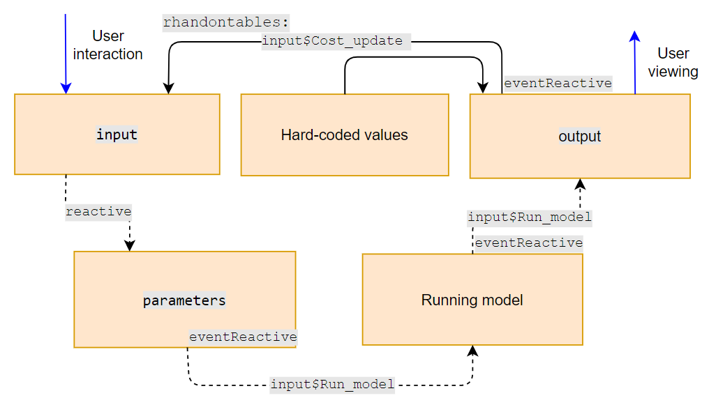
Figure @ref(fig:shiny-model-rhandsreacflow) shows an example of how reactivity in a shiny model could be ordered if a rhandsontable was used to inform inputs. The reactivity would be similar to that presented in Figure @ref(fig:shiny-model-reacflow); however, the hard-coded values do not inform the parameters. Instead, they inform the rhandsontable in the output list, which is then pushed to the input list via the hot_to_r function activated by the input$Cost_update button in an eventReactive. Because this object was required on start-up, a click function was also used that was inside an observe object and was activated if(input$Cost_update == 0). This was the third option on the above list of potential solutions.
Of note, using this method means that an eventReactive object is now upstream of an object produced by reactive, the parameters list. Therefore, to ensure that all the required inputs are available on start-up when the reactive objects are initially made, an is.null is used around the objects that are directly dependent on the rhandsontable, and the hard-coded values inform the input if the rhandsontable does not exist. req would not be suitable here because the rhandsontable is used to produce downstream objects.
An alternative approach would be to have the parameters list also dependent on input$Cost_update; however, using this approach would mean that the input$Cost_update button would need to be selected before clicking input$Run_model, as otherwise the parameters would not have been produced prior to running the model. Having the parameters available on start-up and using is.null requires additional consideration for reactivity, but means that the user will not have to navigate through the model in a particular order.
Code Example 5
This code has the same reactivity as Code Example 4. Before the ‘Run the model’ button has been selected, the ‘Model results’ page now displays a conditional panel informing the user that the button needs to be selected for the model to run. This is controlled by the conditionalPanel function in the ui.R script. Before buttons are selected, they have a value of 0, this increases by 1 each time the button is pressed; once the input$Run_model button is selected it will have a value of > 0, so the results render.
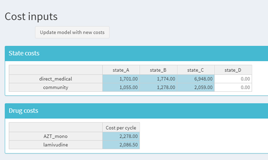
rhandsontable has been used in the ‘Cost inputs’ page to create tables that are user-amendable, unlike the previous versions. Cells which can be interacted with are coloured blue. For the State costs table, State_D is death and in the existing functions there was not the ability for costs to be added after death; as with all models, it is important to only allow user amendable options where appropriate. The tables are defined in the server and are programmed to only be amended with numeric values between 0 and 20000.
Within the server script, the two intermediate objects DM_CC_cost_table_react and Drug_cost_table are eventReactive, dependent on the button to update costs. If the tables have not been rendered then these objects are equal to the base case tables, therefore, the user does not have to visit this page and render this page for the model to work. You will notice however, that this function is dependent on the input$Cost_update button being selected, and there is no guidance on users needing to select this button before running the model. This is because at the bottom of the server script (under the section heading ‘Initial cost setup’) there is the instruction that if the button value is 0, then the button is to be clicked (using the click function). Because the button is activated inside the code, the cost objects will exist when the model starts. This use of the click function could also be used to run the model on model start-up.
The inputs in the ui are not different from the previous code examples, however, conditionalPanel is now used so that the ‘Model results’ page does not render until after input$Run_model is pressed at least once.
tabItem(
        tabName = "tab_Model_res",
        h2("Model results"),
        conditionalPanel("input.Run_model > 0",
                        # Conditional panels are used to render the UI depending on
                         # particular values in the inputs, including action buttons
                         # This "input.Run_model > 0" is only true if input$Run_model
                         # has been pressed
                         fluidRow(
                           box(
                             title = "Model summary",
                             width = 12,
                             solidHeader = TRUE,
                             status = "primary",
                             tags$u("Discounted results:"),
                             dataTableOutput(outputId = "disc_Results_table"),
                             br(),
                             tags$u("Undiscounted results:"),
                             dataTableOutput(outputId = "undisc_Results_table")
                           ),
                           box(
                             title = "Model graphs",
                             width = 12,
                             solidHeader = TRUE,
                             status = "primary",
                             tags$u("Monotherapy trace:"),
                             plotOutput(outputId = "mono_trace"),
                             br(),
                             tags$u("Combination trace:"),
                             plotOutput(outputId = "combo_trace"),
                             br(),
                             tags$u("Comparative trace:"),
                             plotOutput(outputId = "comparative_markov")
                           )
                         )),
        conditionalPanel(
          "input.Run_model == 0",
          # If Run_model has not been selected
          tags$h3("Select 'Run the model' button in Model settings to run the model")
        )
      )
The rhandsontable objects are rendered as an output table in the server similar to as if DT had been used. The cells have been coloured blue in this example to indicate that the cells are user-amendable, and a button has been added to convert the output tables to input values as described in Figure @ref(fig:shiny-model-rhandsreacflow).
The drug_costs object is now dependent on Drug_cost_table, which is an eventReactive object that contains is.null to ensure that if the rhandsontable has not been rendered then the base case values will be used. The eventReactive is triggered on start-up by using the click function dependent on the input$Cost_update not having been clicked previously.
Drug_cost_table <- eventReactive(input$Cost_update,{
    if(is.null(input$Drug_costs_table)) {
      as.data.frame.array(rbind(2278,2086.50), stringsAsFactors = F)
    } else {
      as.data.frame.array(hot_to_r(input$Drug_costs_table), stringsAsFactors = F)
    }
  })

  # ~~ Intermediate cost calculations ---------------------------------------------
  drug_costs <- reactive({
    list(
      AZT_mono = rep(Drug_cost_table()[1,1],input$THorizon),
      lamivudine = c(rep(Drug_cost_table()[2,1],2),rep(0,input$THorizon - 2)),
      combo = rep(Drug_cost_table()[1,1],input$THorizon) + c(rep(Drug_cost_table()[2,1],2),rep(0,input$THorizon - 2))
    )
  })

(bottom of script)
  # ~ Initial cost setup --------------------------------------------------------------
  observe(if (input$Cost_update == 0){
    click("Cost_update")
  })
14.3.7 uiOutput and modules
Sometimes, the value of an input object needs to be reactive and dependent on the value of another input at the same time. For instance, if a certain value from a drop-down menu is selected, then this may be used to populate the options of another drop-down menu or populate numerical inputs to a list of values. In health economic modelling, this is a common need. For example, when switching comparators from an intravenous comparator to an oral one, the relevant options for dosing could change considerably.
This can be achieved by using uiOutput – a placeholder in the ui script for reactive ui elements. The ui object is created inside server using renderUI. uiOutput can refer to single inputs or entire blocks of interface, provided that the content is wrapped within a single block within the ui (for example, tagList and fluidRow are both used in Code Example 6). renderUI can be wrapped inside observeEvent or observe, meaning that it can simultaneously respond to a change in a model input and present the results of a reactive calculation.
Another useful way to control large sections of reactive ui or functionality is to wrap code within modules. This is where sections of the model server and ui are both written as a separate functions, which can then be added or switched between depending on the requirements of the application. An example would be where there are multiple different methods that are each used independently of one other and activated via a switch. Because these can be kept as entirely separate scripts that can be added to models with minimal changes (provided an underlying structure is present), modules are particularly useful if code would be expected to be recycled between models. Because modules are isolated blocks of code, the same input or output objects can be defined and used across multiple modules, and modules can be used interchangeably in this scenario – provided that modules with the same input or output objects are never active simultaneously. Multiple module scripts can be developed and validated, then kept in a library to allow consistent use between projects.
The drawback of using modules is that, as with all functions, objects defined inside modules cannot be used to inform any reference outside the module; this is the case for all input objects. However, like a function, return can be used to output necessary values that can be used elsewhere and referenced in the same way as a reactive object.
As with all objects defined in the server, it is important to consider whether the uiOutput or a module is required at model start-up, and whether or not they exist at the time of use. Any values required from these values on model start-up will require checks using req, is.null, controlled reactivity, or a combination of all three, to ensure that the model does not fail when starting up.
Code Example 6
Looking through the ui.R script, both the ‘Model settings’ and the ‘Model results’ pages no longer have any content aside from the title, a ‘reset settings to base case’ button, and the uiOutput object. Within the server, two additional sections have been added to render both of these pages as output objects. The inputs that are defined within the renderUI object can still be referenced using the input$xxx syntax the same way that an input object defined within the ui.R script is, however there is a difference in that these inputs are defined in the server as output objects and are therefore not available immediately upon start-up. Because of this, all objects referring to these inputs (e.g. input$THorizon and input$combo_HR) that are within reactive or observe functions include an is.null statement which refers to the base case values during start-up. To view this, at the bottom of server.R is an observe statement with a test for whether input$THorizon is null. On start-up the console initially states that input$THorizon does not exist, input$THorizon then renders on the ‘Model settings’ page, then prints that it does exist after the start-up calculations are complete. A second test looks at the existence of input$Cost_update, which is an input on the ‘Cost inputs’ page; the test shows that at start-up this input object exists, even though the page has not been rendered, because this is defined in the ui.R.
There are functions, such as outputOptions, which can make output objects (including uiOutputs) exist before pages render; however these still do not allow the inputs to exist on start-up, so the model will always produce errors if there is a dependency by a reactive object, therefore is.null or req should always be used in these circumstances. Despite these considerations, uiOutputs are a great way of adding flexibility to the model and adapting the input values according to switches or ‘reset buttons’, the latter of which is demonstrated inside this code by using an observeEvent to wrap the renderUI (and click at the bottom of the script to render the ui at start-up).
Within the ui, all of the previous content has been converted to uiOutput("Model_settings_UI") so that they can be re-rendered if the input$Model_settings_reset_button is clicked. Having the settings as uiOutput objects in the server also means that they can be changed dependent on other settings, for instance if there are multiple base cases or adaptations.
tabItems(
      tabItem(
        # ~~ Model settings --------------------------------------------------------
        tabName = "tab_Settings",
        tags$h2("Model settings"),
        actionButton(
          "Model_settings_reset_button",
          "Reset settings to base case",
          style = "color: #fff; background-color: #bd3598; border-color: #2e6da4"
        ),
        br(), br(),
        uiOutput("Model_settings_UI")
      )
Also within the ui, the conditionalPanel has been moved and replaced with uiOutput("Model_results_UI") which is rendered inside the server
      # ~~ Model results --------------------------------------------------------
      tabItem(
        tabName = "tab_Model_res",
        h2("Model results"),
        uiOutput("Model_results_UI")
      )
In the server, the uiOutput is rendered using renderUI. The same syntax is used to create a conditionalPanel, however, the results themselves are rendered inside a module called Results_UI, with the name “ResultsUI”. This demonstrates the flexibility of deriving ui according to the requirements of the model.
  output$Model_results_UI <- renderUI({
    tagList(
      conditionalPanel("input.Run_model > 0",   # Conditional panels are used to render the UI depending on
                       # particular values in the inputs, including action buttons
                       # This "input.Run_model > 0" is only true if "input.Run_model"
                       # has been pressed
                       # Refer to the module UI here, the id of the UI is put inside the brackets. The name can be anything
                       Results_UI("ResultsUI")),
      conditionalPanel(
        "input.Run_model == 0",
        # If Run_model has not been selected
        tags$h3("Select 'Run the model' button in Model settings to run the model")
      )
    )
  })
While these step-by-step points for developing applications should form the foundation of application planning and development, there are additional practicalities that should be considered that are independent of the code itself. These practicalities are introduced in Section @ref(ShinyPract).
14.3.8 Using Reactivevalues lists to centrally manage a shiny app
As the number of uniquely named reactive objects increases, so does the difficulty associated with managing the data flowing through an application. This becomes more obvious when introducing the idea of UI elements containing sets of inputs that move in and out of existence depending on user settings which may or may not exist themselves at any point in time (i.e. nested interdependent UI elements). One way of managing this is to build several independently running modules for different areas of a cost-effectiveness model, using the approaches described in Section @ref(uiModules). This has several advantages in terms of keeping different areas separate and being able to apply namespaces. However, the syntax and cognitive processing involved can make code very difficult to follow, and to convert an existing set of code to use modules can take a considerable amount of time and effort.
An alternative to this approach is to use another type of reactive object, called reactiveValues. A reactiveValues object is essentially a standard R list object (See Sections XXX - Earlier sections in the book about object types), which can house all object types, but exists within the reactive domain. reactiveValues objects are particularly useful because their values can be assigned directly from within an observe or observeEvent. This means that the contents of each reactiveValues element are effectively an expandable and nestable list of reactive objects that do not need to be uniquely named, and do not need defining as reactive or eventReactive. In this sense, one reactiveValues object is like having a data handling module without the additional difficulty of use.
A reactiveValues list, for all intents and purposes, therefore provides much simpler access to a form of namespacing. A particular list containing sub-items has its own name on the top level (e.g. RV for reactiveValues, R for reactive, L for live, D for defaults, and so on), and therefore the items within the list do not need to be uniquely named within the shiny server (e.g. RV$TH could be the time horizon within RV, which could be different to a separate reactive called TH()). When considering a cost-effectiveness model suitable for HTA, one immediately recognises that there may be a requirement for literally thousands of reactive objects to exist to facilitate it in R. This is because a cost-effectiveness model graphical user interface in shiny requires “memory” for elements which may fall out of existence or be refreshed. For instance, in a drug costing framework, one may wish to select how many drugs are included in the model across the various treatment arms, as well as what type of drug each drug is. Each ‘type’ of drug has a different set of required inputs to model cost over time. For instance, flat-dosed treatments do not require information on weight or BSA distribution, whereas IV treatments and banded dosing do. Pill-tracking approaches require another independent set of inputs. Finally, in some more complex situations (e.g. a complex patient access scheme), the user may even want/need to enter cost per cycle directly into an excel-like input area, or even upload an excel file calculating cost over time. As all of these approaches require different sets of inputs, to manually generate them all would result in either a very large and unruly user interface, or a very large and unruly set of R scripts.
This is a common problem that is likely to exist in almost all cost-effectiveness models irrespective of software used to implement them. It is not good practice to simply write out the different user interfaces manually and repetitively, along with large amounts of reactive objects along with isolate commands to let the model ‘remember’ the selections that have been made in the past. Instead, a combination of writing user interface generating code into functions and storing all permutations of data inside of reactiveValues objects provides an easy to use, easy to QC, and almost infinitely expandable platform for building cost-effectiveness models.
The approach we suggest includes a combination of the following four principals:
-
Keep all possible data in a defined set of
reactiveValueslists to allow the Shiny application to “remember” previous selections, and tidy up the flow of data throughout the application. This must include all possible permutations of data in the context of nested and interdependent ui elements (or a mechanism to automatically populate) -
Within the
reactiveValuesobjects there should at least be one that is ‘responsive’, updating instantly when inputs are updated, and another which is ‘live’, updating only when the user commits some changes (i.e. moving the data from the ‘responsive’ object to the ‘live’ object -
Populate all ui elements using the ‘live’ object - this usually requires rendering within
renderUI
In our experience, sticking strictly to these four rules is extremely useful in the context of building cost-effectiveness models in R, when using Shiny as a user interface. It is also an approach which is familiar to cost-effectiveness modelers, in that all data passing through the model passes through a bottleneck which is readable and transparent before being used to calculate results. Finally, one major advantage to this approach is that a model’s state (all inputs and intermediate calculations, and even results) can effectively be ‘saved’ by simply cloning the reactiveValues object describing the current model state (i.e. the reactiveValuesToList() and saveRDS() commands can be used to save an R list containing the state of the model at that time). In the context of interdependent dynamic UIs (See Wickham’s chapter on this here), the ability of shiny to save and load previous states of the application is limited. Shiny uses ‘bookmarking’ to restore the previous state of an application (See Wickham’s chapter on this here). When ui elements are nested and depend on each other, simply restoring the state of objects in the input object is inadequate. For example, if there existed a slider to select a number of drugs included, and a radio button for each drug that currently exists, then restoring the state of the application would restore the slider, which would refresh the buttons, resetting their values to the value they were coded with initially. That is, without a data point to inform the nested elements (which go in and out of existence depending on the higher-level ui elements that control their existence) when they are generated, their values will be ‘forgotten’ by the application upon restoring the application state. This issue is solved using the reactiveValues central data management approach. This is because the ‘live’ object contains data points for all possible permutations of data, irrespective of user selections, and this object never falls out of existence. Thus, it no longer matters if the ui elements are refreshed, their values will be linked to the ‘live’ reactiveValues object. Therefore, simply replacing all of the values in the ‘live’ reactiveValues object will revert the application (as long as the below approach is strictly followed) to a previous state as all data is then the same as it was when the file was saved.
This approach requires some additional groundwork to be laid when making an application, but avoids almost all increases in complication with complication of the application requirements, all whilst preserving transparency and keeping the flow of data ‘tidy’ and under control.
One potential structure for the reactiveValues central data management approach might be:
-
D(i.e. default) -
R(i.e. Reactive) -
L(i.e. Live) -
S(i.e. save)
Where each of the above contain 1st level lists including (for example):
-
basic -
pld -
survival -
drug -
hcru -
utility -
results -
psa -
owsa -
evpi -
etc
Each 1st level list can then contain all information pertaining to that particular theme, and updates to the constituent parts of these objects can be linked to events within the UI of the application (i.e. action buttons to ‘commit’ changes), irrespective of how nested or complex that situation becomes. Equivalently, an entirely different structure can be used to organise model data. However, the above loosely follows the conventional structure which Excel-based cost-effectiveness models follow. For the near future, we expect this to be a structure that health economists in the field worldwide are familiar and comfortable with, so we use it here. The contents of R$basic may be, for instance, R$basic$th (time horizon), R$basic$disc_q (discount rate for QALYs), R$basic$disc_c (Discount rate for costs), and so on, whilst R$pld could house raw and processed/cleaned patient level data (or aggregated analysis results to preserve data security, then requiring a mechanism to load them through), as well as any settings like columns being used for data analysis, covariates, analysis type selections from switches and so on. In other words, keeping all of the information running through the model in one place.
To illustrate further, the list structure of a cost-effectiveness model’s central data object could follow a structure like the one below, where each element below the Root level is itself a list containing multiple objects:
Root
¦--basic
¦--pld
¦   ¦--surv
¦   °--util
¦--survival
¦   ¦--dat
¦   ¦--flexsurv
¦   °--summary
¦--drug
¦   ¦--drug_types
¦   ¦--dosing
¦   ¦--wastage
¦   ¦--cost
¦   ¦--schedule
¦   ¦--subs_tx
¦   ¦--inputs
¦   °--outputs
¦--hcru
¦   ¦--inputs
¦   ¦--schedule
¦   °--outputs
¦--utility
¦   ¦--inputs
¦   ¦--time_to_death
¦   ¦--gpop
¦   ¦--schedule
¦   °--outputs
¦--results
¦   ¦--summary
¦   ¦--detailed
¦   °--ejp
¦--psa
¦   ¦--inputs
¦   ¦--results
¦   °--outputs
¦--owsa
¦   ¦--inputs
¦   ¦--results
¦   °--outputs
°--evpi
    ¦--inputs
    ¦--results
    °--outputs
As can be seen above and in Figure @ref(fig:DRLdiagram), this is intuitive for both those familiar with R and with Excel, and should also be a welcome feature for those that are familiar with cost-effectiveness modeling. Furthermore, as each sub-item in the list structure contains a space for intermediate calculations to be housed, this results in much easier QC and debugging of code.
Example model of controlling data flow in Shiny cost-effectiveness model
In Figure @ref(fig:DRLdiagram), The defaults, D inform live L. Changes to L trigger updates to the UI. Changes to the UI trigger the server, which process and organises the (disorganised) data coming from the UI. The Server now organised information is then passed into R. When D is first inserted into L, once the cleaning process has completed, R should be identical to L, and confirming the changes to update L should trigger nothing. This provides a simple way to test whether the application has started up correctly.
Essentially, D, S, L, and R are complete lists of model parameters, all at different stages. The idea of all parameters passing through one place should be familiar to any Excel-based cost-effectiveness modeller, as a centralised parameters sheet is a very common feature of a typical well-executed Excel-based cost-effectiveness model. The big difference between a parameters sheet within an excel workbook and one of these objects is structure. An R list can contain any number of different types of objects, including live statistical analysis results, numbers, tables, text, Replacing D or L with the saved version S is equivalent to loading a complete previous analysis, meaning that previous analyses can be loaded into the system without closing the application. Note that all of these lists must contain space for every possible permutation of inputs possible in the model, even those that do not exist in the UI at a point in time (for instance if up to 10 drugs can be simulated, the drug input list structure must be laid out for all 10 of them, even if the data elements are just placeholder defaults).
As with initially inserting D into L, when the user changes something in the UI, this triggers actions in the Server which process that information and feed it into R immediately and with a high priority, but does not pass this information into L. At this point in time, R is different to L because the user has not yet committed the changes made to via the UI via a button or some other trigger. When the user commits the changes, the relevant information in R can be placed directly into L. Once L is updated the UI elements that depend on L will update automatically. Their values will correspond to the values of L, whether or not they existed within the UI at the time that L was last updated. This is similar to but more useful than the Shiny command isolate(). This approach can be applied to thousands of data points in one line of code (i.e. L <- R), rather than requiring thousands of individual calls to isolate(). For instance, if the user changes the number of treatment arms from 2 to 3 and commits this change, the potentially thousands of inputs sitting in L for arm #3 will be used to inform all of the inputs for that arm, even if this is the first time that arm was brought into play (and therefore all the inputs for arm #3 didn’t exist at the time). This emphasises the importance of making sure that D contains placeholders for all possible permutations of inputs.
Cost-effectiveness models invariably require a large number of interdependent dynamic renderUI(), especially for the calculation of drug costs, which can follow several different methodologies (e.g. flat dosing, IV medications, dose banding, tracking individual pill consumption). The “DSLR” approach enables a switch to trigger a totally different user interface with different inputs and outputs that are stored and ‘remembered’ separately for any number of independently modeled drugs depending on what type of drug is selected in the UI, without the need for any reactive() or isolate() calls whatsoever.
As discussed above, changes in L immediately change the ui elements directly. Functionally, this works the same way as the updateXXXInput family of commands, but without a need to use them, saving potentially tens of thousands of lines of code. All UI elements are rendered within a renderUI (i.e. server-side) and the value, selected, choices etc arguments for those UI elements refer directly to L, meaning that if L changes, those arguments change, triggering a refresh of those UI elements. However, changing the UI element values should not immediately loop back to L. This is because this would create an infinite loop due to the very small (microseconds) delay between updating a UI element value and the server recognising the change. The user changes a value in the UI, and this triggers the server, updating L, but at the same time the value in L is now different to the value in UI, so the UI is updated to be in line with L whilst the server is still processing the change. Consequently, the server now forever alternates between two values for that UI input. Using R and only updating L via a button or other trigger avoids this. A set of observeEvent calls linked to buttons to populate L using R can be used, whilst another set of observeEvent events update and process R when the UI changes. In short, the process includes the following steps:
-
Outside of the server (typically in global.R): Define
D– the default values.-
For nested or interdependent elements, use
lapplyinside of a function to generate n sets of default inputs, given each selection. This avoids error and keeps the structure ofD,R, andLstandardised -
A more advanced approach could be to generate
nsets of default inputs where n is not the maximumnallowed, and then introduce a trigger (i.e.observeEvent) into the server code which expandsRandLautomatically with default values when the value forninRexceedsninD. However, one must ensure that the values inside ofRare not overwritten with default values when changingn!
-
-
Inside of the server (preferably at the beginning): Define
RandL.-
Due to the nature of the
reactiveValuescommand, one cannot simply enterR <- D. Instead, the 1st level elements need to be passed along. E.g.R <- reactivevalues(Basic = D$Basic). Fortunately, this is just a few lines of code and is quite transparent and easy to read, showing the data being passed along fromDintoRandL. -
Remember if new 1st level elements are added to
D, they should be passed along toRandL. Anything deeper requires no change to the code here. For this reason, it is sometimes worth definingDwith a 1st level entry ofvalsordat(i.e.D <- list(dat = list())). This would mean that passing along toRandLcould just be simplyR <- reactiveValues(dat = D$dat), reducing lines of code a bit. -
Pass along the values from
DintoLas well in the same way -
Now the data in the model matches the data in the default list when the model first opens
-
-
Inside of the server: generate the UI elements, always referring to
Land neverRfor their values-
All ui elements should be generated in
renderUIcalls, and each individual ui element (except for buttons) should refer to an element inside ofLfor its value, selection and any other data that is desirable to store -
Never refer to
Rfor these values, onlyL. This can cause infinite looping and can confuse the process of managing data throughout the application. -
If generating dynamic ui elements, write them into functions, and include an argument for settings, data, inputs etc (e.g.
f_ui_MyUI <- function(n, inputs){<UI elements using n for name generation and inputs for data>}). This lets you pass along the relevant parts of L when rendering the elements for brevity, readability, and efficiency.
-
-
Inside of the server: Track changes in all relevant ui elements, updating
Rand notL-
observeEventshould be used for this. The code is very simple for each input, and we recommend the following: -
observeEvent(input[[<NAME>]],{if(!is.null(input[[<NAME>]])) R$...$<LOCATION> <- input[[<NAME>]]}) -
These
observeEventobservers can actually be defined iteratively within alapplyin the server, meaning they do not need to be typed out individually (an example of this is provided in the code example). Note that you can use the same logic to dynamically generate the names of inputs inside of theselapplyfunctions using thepaste0()command (e.g.paste0(“MyInput_”, 1:n)can be used to generate a set of input names which an then be referred to in theobserveEvent) -
Every input in the entire model needs to be tracked this way (similar to linking parameters through a parameters sheet in an Excel model), which may seem arduous. However, the reward is potentially tens of thousands of less lines of more readable and easier to follow code, not to mention increased computational efficiency.
-
-
Inside of the server: include buttons to update
Lusing values fromR-
This creates ‘choke points’ in the application, using simple and intuitive confirm buttons.
-
Due the nested list nature of
reactiveValuesobjects, different buttons can even be used to ‘commit’ different layers of data. For example, a button could be used to commit all drug cost inputs. This would simply do the followingL$Drug <- R$Drug. This would be equivalent to possibly hundreds of lines of code passing along individualreactiveobjects, in one simple and easy to understand line of code. Equivalently, more specific movements in data can be controlled with buttons deeper into the user interface (e.g.L$Drug$inputs[[2]]$flat$n_unit_sizes <- R$Drug$inputs[[2]]$flat$n_unit_sizescould be passing along just the number of unit sizes available for drug #2, only in the context of flat-dosing. This would then update another nested ui, allowing the user to put in the individual unit sizes, perhaps adding a row to an excel-like table, or another set of numerical inputs). Consequently, the developer has full control over movement of data in the model at this point. -
We would recommend having buttons on several levels to make life easier for the user. One button to commit all drug cost inputs, one to commit inputs for each drug, and anything deeper that’s required should usually be sufficient.
-
-
Inside the UI: simply lay out as normal, using
uiOutputfor the individual elements. -
Create a system to download and upload
L(as an.rdsfile) to allow saving and loading the model state-
As
Ris linked to changes ininputthrough step 4, and changes inLupdateinputdirectly since the ui elements refer toLfor data,Rwill automatically become aligned withL, regardless of how complicated the application is.
-
If these 7 steps are followed, then the cost-effectiveness model (or any other shiny application for that matter) will remain simple in terms of code, no matter how complicated the model becomes. In essence, it will simply be a series of functions which manipulate data stored inside one of two lists, R and L.
One added benefit of this approach is that it allows the developer to interact with the model without using the shiny interface. This is because the default list D has identical structure to the other lists, R and L. Therefore, it becomes possible to step through the calculations that are taking place inside of the shiny application (i.e. by passing data through the event code) without even needing to start up the application. Given a button to download the current state of R or L (or both), one of the main drawbacks of Shiny (difficulty with debugging code) is essentially solved, and the transparency of models can be greatly improved.
Code example 7 (appendix due to length - need to add) follows all steps except 7 and 8, which are just extensions (and only a few lines of rudimentary code). The application provides independent uis for up to 10 drugs, each of which can be one of three types, all with different inputs. Rather than having 30 sets of uis, which would be unruly, the application stores all data in R and L, meaning that it doesn’t matter if some of the UIs are not rendered at some points and exist in others. There are commit buttons for the number of drugs, the type of each drug, and for each individual set of inputs, given the drug type, meaning that the user has full control over the flow of data. Finally, R and L are printed out in real time in the application, allowing full visibility of the model internals with only 3 lines of code each (instead of printing out hundreds of individual inputs). These print outs can be used to observe that changes in inputs immediately update elements inside R, whilst the buttons need to be pressed to update values in L.
The framework for an expansion exercise is built into the code. The object D contains several additional data inputs that are not used. It may facilitate learning to copy the entire script into R and try to expand it by adding more inputs. Some instructions on how to add an input are included in the annotations. Hopefully upon doing this, the advantages of this approach can be seen. Also, it may be worth trying to perform some offline code review by replacing L and R with D outside of the shiny application (literally R <- D, and L <- D and then running through some of the code in the server line by line).
In the example above, R and L are essentially the same. However, in a more complicated context they will begin to deviate from each other. For instance, R will store patient level data and the results of patient level data analysis, whilst L will not as these are not required in order to populate the UI. Although there is some repetition of data between R and L, this is limited as L contains only simple numerical and text information to populate UI elements with. The payoff is full control over when the UI elements will re-render (as this will only happen when the relevant parts of L change), as well as the equivalent of reactive, eventReactive and isolate on potentially thousands of inputs without having to write those lines, invoke any of these operations, or program multi-stage events. The downside of this system is that for simpler applications it is more complicated than simply defining a few reactive objects.
We would recommend that for a cost-effectiveness model a framework consisting of reactiveValues objects is efficient, effective, transparent, and scalable – all of the attributes that model builders and assessors alike seek.
An example: simple drug costing framework
A major advantage to this centralised approach is the ability to pre-populate UI elements with data prior to rendering. This means that even if a UI element does not exist at any point in time, there is always data sitting in the background waiting to be passed along. Let’s say that we want to build in a simple set of drug costing inputs for drug #6, including the following values:
n: How many different unit (tablet, pill, vial, sachet etc) sizes are available for the drug?sizes: What is the quantity of drug within thenunit sizes in mg?costs: What is the price of thenunit sizes in £?unit: By what unit of measure is the drug dosed (e.g. mg/kg, mg/m2, flat-dosed)?dose: what is the listed dose for the drug by the unit as defined inunit
As can be seen, even in the simple drug costing context these inputs all interact with each other, affecting the definition or even existence of the other inputs. The value of n affects how many different numeric inputs are required for sizes and costs, whilst the value of unit affects the definition of dose. All of these changes affect the number of inputs within the UI that is defined for just the parameters defining this one aspect of drug costing. In an excel model, one would simply add another row to a table and drag the scope of the subsequent formulas to include that extra row. In the context of a shiny application, to replicate this, it is necessary to explicitly program the ability to change the definitions and quantity of user inputs on the fly and within the live application. Further still, in a live shiny app there may only be 3 or 4 drugs involved in a particular analysis (e.g. a head-to-head comparison of A vs B with one concomitant drug), meaning that drug #6 does not exist and none of these UI elements are rendered.
There are several approaches to generating said user interface, some of which are simpler than others. Some of the most common approaches include:
- Using
lapplywithinrenderUIto dynamically generate multiple UI elements, depending on parametersnandunit - Using
rhandsontableto housesizesandcostsand allowing the user to add rows to the table, inferringnfrom the number of rows in the table.unitanddoseare presented as a dropdown menu and a numeric input
As this part of the UI is likely to be itself rendered within a lapply within a renderUI, computational efficiency is more important. renderUI can be computationally expensive, slowing down the application. Multiple layers of nesting of this expensive command can then result in a laggy feeling when using the application, with individual elements disappearing and reappearing repeatedly. Consequently, for a feature like the above, we would recommend the second option. This not only simplifies the user interface visually but improves Excel-like familiarity at the same time. Furthermore, it is more computationally efficient and there are less buttons for the user to click, which is particularly important as the server may be rendering e.g. 20 different drugs all with different types of user interfaces to reflect their type. So, in conclusion, our solution to this would be to define a function like so:
# Function: Generates a user interface for very basic drug costing inputs, for
#           a particular drug. Does not take titration, weaning, or dose-loading into account.
#           Does not take drug discounts or RDI into account. Patient characteristic inputs
#           come from somewhere else (i.e. the "basic" element within L)
#           Outputs (inputs) can be used to feed into more complex drug costing
#           calculation steps, thus improving transparency, readability, and the ability to
#           present intermediate calculations within-app.
#
#           Author: Darren Burns
#           Edited: Darren Burns
#           Date  : XX/XX/XXXX
#
#           Drug_n: The number for this drug (e.g. drug #6 would be 6). this determines the
#                   'inputId' argument in all of the individual elements, so that they can
#                   be referenced from the shiny server. e.g. i_drug_drug_basic_n_XXX where
#                   XXX is the drug number entered in this argument.
#
#           drug_name: A label for the drug for the UI, can be pulled from another input set
#                      earlier on, with its own commit button (probably for a UI for names and
#                      drug types, e.g. pills, IV, banded dosing etc)
#
#           hots     : the hands on tables, which must be rendered separately and passed into this
#                      function. This is because handsontables must be directly added to "output"
#                      in shiny.
#
#           I     : The input set to populate the UI elements. I should come directly from L
#                   within the server to avoid infinite looping or other issues. Updates to L
#                   for this sub-element of L should be linked to a button to implement the
#                   changes. Those changes will then feed into R, be processed into the appropriate
#                   form for L, and be passed onto L, triggering a re-rendering of the UI element
#                   generated by this function.
#
#           Rules for I:
#
#           1. n has a maximum value, default of 10. Not many drugs have more than 2 or 3 of these
#           2. The nrow of table is preserved at max_n, irrespective of n. n is used to subset table by row
#           3. unit is one of a set of strings, default is c("mg/kg", "mg/m2", "flat")
#           4. Dose must be a positive number
#
#           Structure of I MUST be:
#
#           List of 5
#           $ n    : num 10
#           $ table: logi [1:10, 1:2] 0 0 0 0 0 0 ...
#            ..- attr(*, "dimnames")=List of 2
#            .. ..$ : NULL
#            .. ..$ : chr [1:2] "sizes" "costs"
#           $ max_n: num 10
#           $ unit : chr "flat"
#           $ dose : num(0)
#
#

func_ui_drug_dosing <- function(drug_n, drug_name, hots, I) {

  # This function has a couple of obvious requirements:
  require(shiny)
  require(rhandsontable)

  # I contains the inputs following the structure defined in the header.
  # As we know the structure already, we can proceed assuming those values
  # exist.

  # all of the other inputs are quite simple. If the user has selected flat dosing,
  # then the dosing numeric input is then just the dose at 100% RDI, and isn't per some
  # measure of patient characteristic.

  if (I$unit == "flat") {
    dosing_label <- "This drug is flat-dosed. The dose is not sensitive to patient characteristics"
  } else if (I$unit == "mg/m2") {
    dosing_label <- "This drug is dosed per meter squared of body surface area (BSA)"
  } else {
    dosing_label <- "This drug is dosed per kilogram of body weight"
  }


  # UI elements:
  #
  # Firstly, a slider to choose how many different unit sizes are available. note the
  # way of naming the input uses the argument to this function, which means easy
  # programmatic generation and reference to it using the same paste mechanism!
  #
  # Note that the max and value arguments come from I, so that L is linked to the UI

  n_slider <- sliderInput(
    inputId = paste0("i_drug_basic_n_", drug_n),
    label   = paste0("Number of different unit sizes avaialble for ", drug_name),
    min     = 1,
    max     = I$max_n,
    value   = I$n,
    step    = 1,
    ticks   = TRUE,
    width   = "100%"
  )

  # Next, an rhandsontable for the table. By preventing the context menu this
  # prevents the user from adding rows to the table. As the slider above has already
  # looped round and changed I$n, this means that the number of rows in this excel-like
  # table should not be editable!

  hot <- rHandsontableOutput(hots)

  # Now a dropdown menu for the basis of dosing. Includes an option for flat
  # dosing, meaning that the denominator for dose_num below is either kg, m2 or
  # nothing.

  unit_picker <- selectInput(
    inputId = paste0("i_drug_basic_unit_", drug_n),
    label   = paste0("Basis of dosing for ", drug_name),
    choices = c("mg/kg", "mg/m2", "flat"),
    selected = I$unit,
    multiple = FALSE,
    width = "100%"
  )


  # next, a numeric input for dose. This is per characteristic unit, or just flat
  # depending on option in the dropdown menu above, either way its stored in
  # the same place. The dropdown option determines which function the data
  # generated here feeds into (i.e. directs to the appropriate way of costing
  # up the drug). note that the label is determined by I$unit, allowing the user
  # to easily see in the UI what information they are entering into the model.

  if (I$unit == "flat") {
    dose_numeric_label <- paste0("Dosing for ", drug_name, " (fixed)")
  } else if (I$unit == "mg/kg") {
    dose_numeric_label <- paste0("Dosing for ", drug_name, " (per kilo)")
  } else {
    dose_numeric_label <- paste0("Dosing for ", drug_name, " (per m2 of BSA)")
  }

  dose_numeric <- numericInput(
    inputId = paste0("i_drug_basic_dose_", drug_n),
    label   = dose_numeric_label,
    value   = I$dose,
    min     = 0,
    max     = Inf,
    width   = "100%"
  )


  # Finally, a button to confirm the user selections for this drug for this drug type
  # for this arrangement of inputs.

  confirm <- actionButton(
    inputId = paste0("i_drug_basic_confirm_", drug_n),
    label   = paste0("Confirm inputs for ", drug_name),
    icon    = icon("calculator"),
    width   = "100%"
  )

  # put all these bits together inside of a panel so that the panel can be positioned
  # higher up in the stack. A function called tagList() makes this easy

  ui_output <- shiny::inputPanel(
    fluidRow(
      width = 12,
      column(
        12,
        tagList(
          "The below inputs control the dosing for ", drug_name, ". Please confirm the ",
          "number of drugs first using the slider and button, then enter the other inputs.",
          br(),
          confirm,
          n_slider,
          hot,
          dose_numeric
        )
      )
    )
  )


  # return the final UI
  return(ui_output)

}


func_ui_drug_dose_table <- function(I, drug_n) {

  # limit the table to go to the UI to only the rows 1:n so that if user has chosen
  # value n < max_n then it won't show the rest of the table. Note that changing
  # the user input for n without saving changes first will overwrite the UI inputs.

  tab_d_c <- I$table[1:I$n,]

  # now generate a hands on table
  hot <- rhandsontable(
    data       = tab_d_c,
    colHeaders = colnames(tab_d_c),
    search     = FALSE,
    width      = "100%"
  )
  hot <-
    hot_table(
      hot = hot,
      highlightCol = TRUE,
      highlightRow = TRUE,
      stretchH = "all",
      contextMenu = FALSE
    )
  return(hot)
}
With this function defined, it becomes much easier to generate the e.g. 20 different drugs which may be included in a cost-effectiveness model:
As the inputs generated within these UIs are only linked to L in one direction (fro L to UI), they must be linked up to R, and then the confirm buttons must be linked to feed the values from R into L:
# Also in the server, define observers which watch all of the inputs, and update the values
# inside of R. Also define the update buttons and the event to move data from `R` to L

for (drug_n in 1:L$drug$basic$max_n) {

  # the hands on tables - render the table for this arm so it can feed into the renderUI:
  output[[paste0("ui_drug_dosetable_", drug_n)]] <- func_ui_drug_dose_table(I = L$drug$dosing[[drug_n]], drug_n = drug_n)

  # sliders. for this drug, watch the slider for unit sizes, and whenever the user
  # changes the slider, update the value in R, but not L. Value is stored but not
  # causing the UI to repeatedly refresh itself because it only depends on L. give
  # this a high priority to make sure it happens before other responses.

  observeEvent(input[[paste0("i_drug_basic_n_", drug_n)]], {
    if (!is.null(input[[paste0("i_drug_basic_n_", drug_n)]])) {
      R$drug$dosing[[drug_n]]$n <- input[[paste0("i_drug_basic_n_", drug_n)]]
    }
  }, priority = 100)

  # tables - convert them back to standard `R` objects so they can feed into `R` properly:
  observeEvent(input[[paste0("ui_drug_dosetable_", drug_n)]], {
    if (!is.null(input[[paste0("ui_drug_dosetable_", drug_n)]])) {
      R$drug$dosing[[drug_n]]$table <- hot_to_r(input[[paste0("ui_drug_dosetable_", drug_n)]])
    }
  }, priority = 100)


  # units:
  observeEvent(input[[paste0("i_drug_basic_unit_", drug_n)]], {
    if (!is.null(input[[paste0("i_drug_basic_unit_", drug_n)]])) {
      R$drug$dosing[[drug_n]]$unit <- input[[paste0("i_drug_basic_unit_", drug_n)]]
    }
  }, priority = 100)

  # Dosing
  observeEvent(input[[paste0("i_drug_basic_dose_", drug_n)]], {
    if (!is.null(input[[paste0("i_drug_basic_dose_", drug_n)]])) {
      R$drug$dosing[[drug_n]]$dose <- input[[paste0("i_drug_basic_dose_", drug_n)]]
    }
  }, priority = 100)

  # Confirmation buttons: the action in this one is simply to pass along the inputs
  # of interest to L from R. this gets highest priority to make sure it happens
  # right away and before any rendering triggers for L into the UI.
  observeEvent(input[[paste0("i_drug_basic_confirm_", drug_n)]], {
    L$drug$dosing[[drug_n]] <- R$drug$dosing[[drug_n]]
  }, priority = 150)

}
Now, irrespective of how many drugs are included in a model (up to the maximum L$drug$basic$max_n), as long as there is a space for them inside of R and L they can automatically be rendered within the UI. The values of these will not be “forgotten” if a user changes L$drug$basic$n, and the use of a confirmation button prevents unnecessary repeated processes. Following this workflow allows for a transparent and easy to expand application that can be debugged without running the server, and all inputs in the entire model can simply be saved by saving L as an external file or on a server (e.g. saveRDS(reactiveValuesToList(L), "./debug/L.rds") would save the entire list L as an external file, allowing full review and transparency). This approach then allows review of the inner workings of the Shiny application outside of the shiny server, as one would simply save a copy of R or L into a file, load it back into R without the Shiny application running, and then step line by line through the desired server code. Finally, the object R can also house the results of intermediate calculations (which are not required to populate L and therefore not passed along to it), which can then be presented back to the user in the UI for QC or review. This can include elements of automated QC like checking whether the overall survival hazard of a patient population falls below that of the general population, whether any costs are negative and so on.
Overall, this method is conducive to transparency, repeatable even in the context of Shiny, and scalable to any level of app complication.
14.4 Practicalities of building a shiny application
14.4.1 Overview
This section focuses on the real-life practicalities involved with building the kinds of useful shiny applications that would be required in the world of HTA.
A discussion of the acceptability of shiny for HTA is provided in Section 14.4.2.1. This discusses visual vs logical programming interfaces, and their acceptability within different HTA processes around the world. Following this, the acceptability of R/shiny in future HTAs is discussed.
Understandably, HTA processes around the world tend to have a focus on transparency and fairness. shiny applications are interactive, flexible, efficient, and can rely on externally validated functions to allow validation. Yet, the ability to click into the cells of an Excel-based cost-effectiveness model and see not only the flow of data and dependency, but the individual blocks of code interacting is difficult to replicate in any other software. Whether this interactivity is truly transparency, or we health economists are just “used to” the often extremely high level of unnecessary difficulty and inconvenience involved in reviewing Excel-based cost-effectiveness models is unclear. Yet, a shiny application can also be built in a profoundly opaque way, potentially with the user interface being just the results. However, there are several strategies that one can leverage when building a shiny cost-effectiveness model, which can ultimately provide a high level of true transparency (see for example our tutorial in the online version of this book). This is discussed further in Section 14.4.2.1.
R is a foremost a statistical language, and so the topic of shiny applications to present an interactive statistical analysis is provided in Section 14.4.3.
Following these top line discussions, a more detailed description of our recommendedations on organising a shiny application is provided in Section 14.4.4. This is followed by a discussion of user interface layout in Section 14.4.6.
One major advantage of using R is data security. Excel models, particularly those including extensive VBA code are not easily hosted online, and their interactivity usually means that any sensitive data contained therein is easily accessed. As R has packages for secure database access, and shiny applications can be hosted on the cloud, this can avoid this issue completely. Section 14.4.7 discusses this in more depth.
Finally, one of the most important advantages of using a programming language like R to build a model is the fact that the model itself is fundamentally a set of plain-text scripts. As such, increasingly popular version-control programmes like git and GitHub can be used to gain access to proper version control — something which is not possible with many other software implementations. Version control is ubiquitous in the software development world and for good reason. A folder of hundreds of superseded files is a thing of the past and a record of who made what changes when and for what reason is generated throughout the development process, providing accountability and a timeline. The process of QC becomes continuous and much more robust in comparison to a full QC at the end of the process, which can often take many days of remembering changes that occured months earlier. Our recommended process for version control for the often small teams of developers working on cost-effectiveness models is provided in Section 14.4.8.
14.4.2 HTA requirements
Current acceptability of shiny within HTA
A model implemented in shiny lies between primarily visual programming interfaces like TreeAge and purely code-based models such as those implemented entirely in Microsoft Visual Basic for Applications (VBA). In this sense, they are not dissimilar to Microsoft Excel, which also combines graphical interfaces with programming. shiny offers a middle ground, where the modeller can easily demonstrate visually that their calculations are correct through presentation of intermediate calculation results, but also has access to the broad range of statistical analysis options and computational efficiency that R can offer.
In the visual modelling case, the underlying programming must be trusted unequivocally as it is closed-source. This precludes critique of the code underpinning the functions (e.g. the code underpinning functions like SUMPRODUCT, MMULT, INDEX and so on) to calculate the model results, limiting model critique to what can be seen in the graphical user interface (GUI). Models of this nature are widely accepted across HTA bodies and have been for many years. Conversely, models implemented entirely in a code framework with no GUI are often cast in a negative light due to a lack of transparency, despite every calculation in the model being exposed for review, even those which would not be exposed in a graphical implementation. Depending on the definition of transparency, this could be perceived as much more transparent than an Excel-based model, as Excel functions are implicitly assumed to be correct without review of their underlying code (which is closed-source and therefore cannot be audited). However, the attitude to code-based models in HTA has been gradually softening in recent years, and there are several examples of code-based models implemented in VBA being accepted by NICE and evidence assessment groups (EAGs). NICE EAGs and the NICE guidelines team have also been producing models in R for use within HTA including use of Shiny within a recent asthma diagnostic guideline (Guideline, 2024; Lee et al., 2024).
That being said, when we inquired in 2024 (Table 14.2) not all HTA bodies currently accept R including shiny as a platform for appraisal of the cost-effectiveness of a product and those that do require advanced notice, justification for additional complexity and in general prefer Excel. The responses from HTA bodies consulted are listed below.
shiny (as of April 2024)
| HTA body (country) | Attitude towards shiny |
Reasons stated |
|---|---|---|
| NICE (England & N. Ireland) | Accepted | Per NICE manual |
| SMC (Scotland) | Accepted | Accepted provided there are no password or access control issues. Excel preferred |
| NCPE (Rep. of Ireland) | Accepted | Providing notified in advance, complexity is justified, guidelines are followed, code is well annotated and intermediate calculations are presented in shiny. Excel preferred |
| CADTH (Canada) | Accepted | With prior agreement only |
| ZiNL (Netherlands) | Accepted | Recent successful pilot of use of R and Shiny within a ZiNL submission for oncology has been complete |
This is likely to change in the future with the increasing need for flexibility and statistical analysis within cost effectiveness models.
Future acceptability of shiny in HTA
The use of Shiny within HTA is expected to increase given the uptake of R for medical statistics and within HEOR and NICE Committee feedback on the usefulness of the Shiny Interface to allow live scenario testing to inform decision making. Some features which R/shiny brings to the table with respect to usefulness for HTA include:
- The prospect of end-to-end functionality, or the ability to go from patient data to cost effectiveness results all in one place. This then allows a more iterative approach to HTA decision making. When a set of assumptions has been chosen and new data becomes available, the analysis can simply be rerun, producing new results in a report format automatically. This will be increasingly important as plans for more frequent reevaluation and even real-time decision making come to fruition
- The improved security and reduced probability of leaking sensitive data involved with remote hosting. Access to the application can be given to reviewing bodies as an alternative to sharing files containing sensitive data.
- The ability to explicitly incorporate QC processes into models via a form of “unit testing”. This can be achieved through inputting a standardized set of model inputs for every model (to be made publicly available and depending on structure), and expecting the model to then produce a pre-calculated set of deterministic and probabilistic results. Deviations form this result can either be explained by the deviations from the case for the test dataset or accepted to be the result of errors. Either way, the process is far more transparent than the status quo of large
Excelmodels containing potentially hundreds of thousands of manually entered formulae - The potential for standardisation: the calculations required for the disease model of a three-state partitioned survival model with no additional or tunnel states will always be the same, and nothing prevents HTA bodies from endorsing efficiently programmed and validated standard
Rfunctions - The advantages of the ability to make use of version control software to more easily allow and track stakeholder interaction with models and create HTA code repositories
- Interactivity of graphics: a nice feature of
shinyis its ability to utilise HTML and javascript, which have many ways to provide visual feedback to users. This means that features like interactive plots, tables which can be saved for validation purposes, elements which can be tucked away or expanded without the need for macros are all a possibility. The potential for this to greatly simplify the process of understanding, reviewing and making decisions using a cost effectiveness model is great, given our industry learns with the right paradigm of simplicity and transparency.
14.4.3 shiny in HEOR and medical statistics
More broadly in the health economics industry as well as in medical statistics, there is some uptake of shiny for earlier steps in the regulatory and market access pipeline. This includes:
- Tools for feasibility assessment and early cost effectiveness modelling
- Value tools to be used in the field during direct contact with clinicians
- More broadly in medical statistics and analysis and visualization of epidemiologic data such as the spread of the Covid-19 pandemic (for example, GSK, one of the leading pharmaceutical companies, are using
R,Rmarkdownandshinyfor medical statistics)
In the professional consultancy and academic worlds, we have seen demand for such products increasing, and are reacting to this incentive to train our staff in the use of R and shiny. We see this as being an investment in the future of the industry.
Within the academic world, there is much scope for the use of automated reporting and interactive research. The ability to run and see the details of scenarios which are typically described as a sentence or in a table within a journal article is just one way that the research presented within a journal article can remain succinct whilst making all facets of its results available to readers. There is also the prospect of self-updating research, within which quantitative research is updated when new data becomes availabe, the authors are notified and can update their conclusions. This is an exciting prospect for trial publications, which often reach publication before the end of patient follow up.
The idea of interactive research may be a somewhat daunting prospect for academics, who are exposing their work and inference to continued scrutiny by allowing readers to engage with their analysis directly. However, this is simply an extension of the peer-review process already ubiquotous in academic publishing. Given proper channels and processes to allow peers to engage with and comment on previous research increases the exposure and therefore impact factor of the research itself, and may even permit citations that would otherwise not been made. One notorious example in the HEOR consultancy world is the study by Ara and Brazier (2011) on UK population norms for health-related quality of life. This was used for many years as standard for NICE submissions in the UK to adjust for the gradual decline of quality of life as people get older. However, the study (which uses a regression analysis) does not present a variance-covariance matrix, preventing using a multivariate normal assumption making probabilistic draws for the parameter values which take their correlation structure into account. Had this study presented a shiny application or even an automated report, it would have updated this regression analysis upon new rounds of data becoming available, but would have also provided a platform for the variance-covariance matrix to be presented without taking up unnecessary space in the journal article.
Another benefit of shiny applications and automated reports (e.g. using bookdown or quarto to produce the article) is that appropriately aggregated data can be made avaialable directly. This may completely preclude the need for digitization of Kaplan-Meier raster data (see Chapter 7), as the report can produce exact Cartesian co-ordinates, or even exact anonymised time and event data (just event times and event/censor values). This allows exact replication of the Kaplan-Meier analysis, which is invaluable for HTA.
The QALY shortfall tool made by ScHARR alongside industry contributors is a live example of this. This was published alongside a shiny application, allowing the reader of the article to test out values and gain estimates relevant to their own HTA submission, directly using the precise methodology proposed by the authors. As the authors have made this tool themselves and used it to present the results in the article, there can be no question that the values in the article and the application are aligned. This provides an exciting prospect for academics — that the result of their research effort is not only their proposed method and a journal article, but also a usable tool which will be widely used within the HEOR world for years to come.
14.4.4 Framework
The framework of a shiny application presenting a cost-effectiveness case for a clinical intervention should be as organised as possible. Putting the entire application in one script which is not associated with an .Rproj file is unlikely to be comprehensible by any reviewer, as it is likely to be a monolithic script containing tens of thousands of lines of code with no real structure to it. This is analogous to an entire excel model being placed within one worksheet with no formatting to the individual tables, which would of course be unacceptable.
We recommend designing and implementing a structure for the different scripts of the model which is both familiar to you and conducive to exogenous review. In this section, we provide some recommendations on the structure of a shiny application performing a cost-effectiveness analysis based on our experience (that is, our past mistakes).
Overview
Variety in organisational structure of cost-effectiveness models is to be expected and to some extent encouraged in order to promote innovation and better solutions going forward. Yet, standardization of structure is also extremely useful for review and efficient QC of models. Reviewers having pre-knowledge of where to look and what to read to follow model calculations can save considerable time, and more importantly allow them to focus on the health economics rather than convoluted mechanics and information retention. Excel model reviewers likely understand the importance of this, as poorly laid out Excel-based cost-effectiveness models can be notoriously difficult to follow - even if the cost-effectiveness model itself if conceptually simple. This issue is exaggerated by orders of magnitude for entirely code-based cost-effectiveness modelling, where the model is essentially a collection of plain text files and some data, not housed within the same file, folder, style, structure. Consequently, structure, explanation, and organisation are far more important than in any other implementation.
The Decision Analysis in R for Technologies in Health (DARTH) group have published recommendations for structuring cost-effectiveness models in R. (Alarid-Escudero et al., 2019) These suggestions include naming conventions, computational structure, folder structure and even unit testing. We mostly agree with the proposed structure in this article, but have developed our own position on overall structure which deviates from this slightly — particularly with issues of handling thousands of data points (see our tutorial in the online version of this book). However, this deviation highlights one important point - just as with models implemented in any other software, code based models will vary in the way that they are organised. The important thing to recognise is that a model will be easy to follow if:
- It follows a framework that is documented, intuitive, and easy to follow
- The parameters are named consistently and transparenty
- Functions are defined in place of repetitive long pieces of code
- There are extensive annotations throughout the model, particularly on functions explaining what is happening and why
- The functions used are not closures (functions without arguments e.g.
myFunction())
Always use R projects
One of the biggest differences between a model based in a programme such as Excel and a model based in code is that a code-based model is typically composed of multiple files, which can be organised in any number of ways. Within a shiny application, which requires server and user interface components, this number of scripts can very quickly become unruly without proper organisation. Although this sounds daunting, the process of keeping files organised is actually rather simple in our experience. We advise that shiny apps are always made within an R project, for the following reasons:
– Rstudio or the Rstudioapi package can automatically identify the working directory, wherever that is on the computer – Applications can easily be shared and will always work, even if copy pasted – Applications can easily be version controlled using git or SVN – The references to different files can be relative (e.g. ./ for “this folder”, ../ for “the folder above this one”)
The advantages of housing projects within R project folders are so overwhelming that we suggest that every piece of work in R should always be done as an R project.
Folder and script filing structure
shiny apps can be arranged in one single script, or can be broken down into multiple scripts according to some framework. We recommend the latter, as although the code for shiny apps is mostly simple, the number of calculations required for an economic model are such that one single script would be unruly. For instance in a demonstration model we made to demonstrate the usefulness of R/shiny in cost effectiveness analysis, the application was approximately 40,000 lines of code in total. In that instance, the application was split up into one ui script for each tab in the dashboard (similarly to an Excel model). The server scripts in this application were split by computational node within the cost-effectiveness model. However, as the tabs themselves are already thematic in nature, further consolidation led to some confusion during model construction and finalisation.
Following this experience, we now recommend that the ui and server scripts are both based on the tabs in the dashboard. This may mean that some could potentially be empty whilst others are long or potentially themselves parent files which source smaller files (e.g. server_dcost, which sources several other files like server_dcost_nametype, server_dcost_dosing, server_dcost_schedule to define the functions related to drug costs). This may seem contrived, but the structure is clear and intuitive, and finding particular elements or calculations is trivial.
The UI and server scripts are organised into their own folders, and these can contain their own sub folders. This ensures that within the project, everything has a space of its own and no script becomes unruly. Due to the “search in all files” (ctrl+shift+F) and “go to anything” (ctrl+.) features in Rstudio, finding things is very easy, even in large file structures like these, allowing a similar process to “trace dependents” in Excel.
DARTH suggest a folder structure to use for cost-effectiveness models. (Alarid-Escudero et al., 2019) We have used several different folder structures in our previous cost-effectiveness endeavors in shiny, and have arrived at a similar folder structure to the structure proposed by DARTH for cost-effectiveness models which is slightly modified for shiny applications:
├── data
│   ├── global.R  <- Default inputs for switches/buttons/ inputs at runtime
│   ├── raw       <- Original, raw data; may not exist if data from internet
│   └── processed <- Processed, cleaned data - likely not used here
│
├── docs          <- Documentation for internal use
├── outputs       <- Generated outputs (reports, figures, etc)
│
├── report        <- Write up for external use. .Rmd/.qmd/.bib files
│
├── src           <- Source code for use in this project - subfolders by theme
│  ├── utils      <- Generic utility functions
│  ├── basic      <- Basic data processing (time horizon, discounting, etc)
│  ├── surv       <- Survival analysis functions
│  ├── dcost      <- drug costing functions
│  └── ...        <- other subfolders
│
├── tests         <- Tests for this project - e.g. testthat.
│
├── app_files     <- Folder for Shiny App content, includes file app.R
│  ├── app.R      <- The main `R` script for running the shiny app
│  └── UI         <- folder with UI content.
│     ├── ui_master.R
│     ├── welcome
│     ├── Basic
│     ├── surv
│     ├── dcost
│     └── ...
│  └── server     <- folder containing server file
│     ├── server_master.R
│     ├── welcome
│     ├── Basic
│     ├── surv
│     ├── dcost
│     └── ...
│  └── www        <- other content.
│
├──.github
│  └── UI         <- contains all workflows for github actions
│
├── .gitignore
├── LICENSE
└── README.md     <- Top-level README (for github/gitlab repository)
This structure is similar to the structure required for standardised R packaging, and can be adapted to fit with that, which allows the shiny application to be packaged up so that it has proper help files, vignettes, code-completion prompts and other useful features. It also means that unit testing via the testthat package can be introduced, also in line with DARTH’s suggestions.
The above sounds complicated, but is in fact very simple and easy to follow. In the above folder structure, the script app.R would look something like this:
# Example application

# load the UI and server:
ui     <- source("../app_files/UI/ui_master.R")
server <- source("../app_files/server/server_master.R")

# run the shiny application
shiny::shinyApp(ui = ui, server = server, onStart = source("../data/global.R"))
This loads in the user interface and server, and the raw data via global.R, and then runs the application. This would never change, irrespective of the underlying structure of the application. Within the scripts ui_master.R and server_master.R there will be several source calls to the files under these in the hierarchy, and this can continue infinitely until the individual scripts involved are all broken down to a reasonable size that is easy to read.
Whether or not the DARTH folder structure framework, one which is more adherent to R packages, or another structure entirely is used should be considered carefully alongside model conceptualisation. In effect, this is a different “kind” of conceptualisation, revolving around the mechanics and logistics of the framework the model is going to be built within.
From the start of a project of this size (and especially prior to a large undertaking requiring many layers of complex interplaying logic like a global cost-effectiveness model), it should be made clear whether or not the model or analysis will ultimately end up becoming a piece of software unto itself. If that is the case, and it is unlikely that a user will need to directly edit the functions defined in the project during an adaptation, this is more conducive to becoming an R package.
On the other hand, if the code is useful in terms of re-usability but would require some bespoke additions or edits, then generating an R package will ultimately limit the reusability of the code that is written. This would be similar to an excel file you can re-use but you cannot edit the formulae inside of the cells, limiting its usefulness.
Furthermore, it would be highly unusual to compile a specific statistical analysis (as opposed to a generalized set of methods to conduct that analysis) into an R package. This is because a bespoke analysis of some specific data is not a software, but rather an analysis. Yet, the methods used in that analysis (if generalisable to other use-cases) are exactly what R packages are intended for. Shiny applications performing a type of statistical analysis then lie in a grey area between these two contexts, leading to some debate on which is the most appropriate way to publish them.
Consequently, it is more important than it might initially seem to define whether the project you have in mind is a bespoke analysis that can be adapted for future use, or a software that can be used repeatedly. That decision directly influences the most useful way to store, update and share the code. Ultimately, it determines whether it is more useful to compile the project into an R package to be downloaded and installed as a part of the suite of R packages used for statistical analysis, or to organise it in another way which makes it easy for people to adapt without losing confidence in the integrity of the code it contains (which is the intention of the DARTH framework).
That being said, there is nothing preventing one from organising the code following the structure of an R package, but stopping short of compiling the package into one. Doing this can be useful, because one can compile the code as a package to conduct unit testing and render all of the documentation to check things are working correctly, but publish the code prior to that compilation (or compile the package in a git branch, or even vice versa!). This strikes a balance between reliability, re usability, adaptability, and transparency which is more conducive to cost-effectiveness modelling in health economics and is less geared towards statistical analysis methods.
Overall, an important choice should be made before building your shiny application, conducting your statistical analysis, or even during conceptualisation around what the result of the work will ultimately be. Will it be software, analysis, or a set of methods? Will it be all three?
14.4.5 Naming conventions
R scripts in shiny applications are usually divided into many different scripts based on purpose, and the objects that are created, processed and presented during the calculation process can often change names and locations multiple times during the process. It is therefore very important to be organised, clear and deliberate when naming files, objects, and even indices used within functions or iterative processes.
Files, objects and indices should be named according to a system, not on a whim. This seems like an easy corner to cut, but in our experience the net increase in modelling time required from not naming files and objects in R code according to a set of conventions is considerable due to the errors caused. When a script has literally thousands of objects being defined in it across tens of scripts, naming a looping index or an object x is simply not good enough. It will invariably be lost in the code, and may even get confused with other objects called x causing errors. Instead of this chaos, we recommend the following:
Files:
Name files inside server, u and module folders with server_, UI_, or module_ as a prefix to the filename. This way it is obvious what a file’s purpose is not only from its location, but also its name. This is very helpful when working in a programme such as Rstudio, and when having 10+ files open at the same time whilst trying to build in a new feature. The same is true of suffixes as well, which should also be standardised.
Objects inside scripts:
As with file naming prefixes and suffixes are extremely important in keeping things consistent within scripts. This can help prevent errors before they happen. For example, shiny inputs and outputs which go to and from the UI could have the prefix ui_ at the beginning of their names. This makes the reader immediately understand what the object is for. Also, if prefixes and suffixes are standardised, this allows iteration across different parameters using the paste0 function in R (Chapter 2). For instance, if there are 10 drugs in a model and the dose in mg per unit of patient characteristic is named i_dcost_dosePerChar_drugx where x is the number of the drug, then one can find the input inside of the input object for drug 5 like so: input[[paste0("i_dcost_dosePerChar_drug",5)]]. As the “5” can itself be another input (e.g. “use dosing from another drug for this drug”), this allows programatic links between inputs, which is far more convenient than having to memorize differently structured names for objects.
It is obvious from i_dcost_dosePerChar_drug5 that it is: - A model input (because of i) - Part of the drug costing framework (because of dcost) - providing dosing per patient characteristic value (per kg, m2 of weight, because of dosePerChar) - specific to drug number 5 (because of 5)
This name is long, but descriptive. Names like x or i_dc_dpc_5 are clearly more succinct for a human to read, but also require more memorisation for us to comprehend. This pulls concentration away from the act of reading the code. By contrast, a computer does not care how long a parameter name is and the difference in reading time is measured in small numbers of nanoseconds between very long and very short names. Yet, lots of long names one after the other can become irritating to read, which has certainly been the case in some of the previous shiny applications made by the authors of this chapter. This is yet another reason to centralise data inside of a reactiveValues list structure, as discussed in the tutorial for the online version of this chapter (see the book online website https://gianluca.statistica.it/books/online/rhta). A similar call to a parameter within the DSLR structure may be R$dcost$dosePerChar[[5]], which is no different from i_dcost_dosePerChar_drug5 in length. However, in practice, code is often simplified before individual inputs are used:
# get dose per characteristic measure for all drugs:
dosePerChar <- unlist(R$dcost$dosePerChar)

# Now use dosePerChar in subsequent calculations:
Without the consolidated list structure, this would need to be a process involving compilation of all possible strings i_dcost_dosePerChar_drugx, pulling them from input one by one, then feeding them into the next calculations. With a consolidated list structure, it’s just a case of pulling out the appropriate organised data, simplifying the code where more complex calculations may be taking place considerably. The other advantage is that the names of the items with in the list do not need to be memorized, as one can just press tab or use names() or str() in R to be reminded. When a shiny application is as big as a HTA-ready cost-effectiveness model, this is invaluable.
In conclusion, conventions and processes for naming or structuring data in code are essentially very similar ideas. Nested naming conventions are useful for programing and automating tasks in a similar way to structuring the data in a way that makes that unecessary. Typically both will need to be used in order to be able to stay organised in the face of a cost-effectiveness model.
Indices
Indices within an iterative operation are no exception from the importance of naming things in a way that can be understood. For instance in the simple example lapply(1:3, function(i){lapply(1:5, function(j){unlist(lapply(1:2, function(k){lapply(1:1000, function(l){...})})) + 1})}), interpretation of k during a review is unnecessarily difficult. However, if these indices had descriptive names like arm, drug, dose_phase, model_cycle, the intention of the operation becomes considerably clearer.
We advise that descriptive index names should always be used, and x, y, z, i, j, k should be avoided as much as possible.
Computational efficiency
One complaint that we have seen about R, and have experienced in our early efforts with shiny is that it is slow. R is a vectorised language, designed to perform matrix algebra very efficiently. Consequently, any kind of vectorised operation (such as element-wise multiplying one column by another like a * b, or matrix-multiplying them to get the Excel-equivalent of SUMPRODUCT like t(a) %*% b) are very efficient in R, and can be used to improve the computational efficiency of a cost-effectiveness model. Similarly, R is extremely fast at working with the matrix class of object, far moreso than other common classes like data.frame. Big calculations like those taking place in patient flow sheets should be done using matrices and as efficiently as possible. We have experience of adapting an existing R-based cost-effectiveness patient-level simulation model, during which time we improved computational efficiency around 1200x (from 200 patients in ~120 seconds to 20,000 patients in ~10 seconds). As we also imposed a structure similar to those described above, the model was far easier to follow as well. In conclusion, efficiency does not come at the cost of readability, and is very important to consider in cost-effectiveness models, which contain a lot of interdependent calculations.
One of the most important functions for improving efficiency we have found is Reduce, which is in base R so doesn’t require other packages to be loaded (Chapter 2). This function is invaluable for cost-effectiveness models which use discrete time steps. This function is similar to lapply, but with the important difference that it refers back to the result of the previous iteration. Due to this, it is very useful for calculating traces, and can be used to calculate a patient flow sheet one entire row at a time (similar to dragging down a lot of formulas at once in Excel). Naming conventions are very important in these Reduce environments because it is easy to become confused as to what one is referencing, be it an object or an index. The most likely application in health economics cost-effectiveness modelling is best described by the example below, which produces Figure 14.1:
library(ggplot2)

# A population starting in state 1 is exposed to matrix 1 for 5 cycles
#   and matrix 2 for the rest of the model until the time horizon
Starting_states <- c(1, 0, 0)

# first matrix is applied for N cycles (i.e. cycles 1-N)
#  Note that cycle 0 doesn't count
Switch_TPM <- 5

# time horizon
Time_Horizon <- 49 # Cycle 0 is described by Starting_states so 49 for 50 total

# Transition probability matrices (TPMs)
TPM_1 <- matrix(
  c(
    0.85, 0.10, 0.05,
    0.05, 0.80, 0.15,
    0.00, 0.00, 1.00
  ),
  ncol = 3,
  byrow = TRUE
)
TPM_2 <- matrix(
  c(
    0.80, 0.10, 0.10,
    0.01, 0.80, 0.19,
    0.00, 0.00, 1.00
  ),
  ncol = 3,
  byrow = TRUE
)

# use Reduce to repeatedly apply the matrix to the result of the
#   previous calculation, with the condition of changing the TPM
#   after applying it N times
StatePopList <- Reduce(
  x           = 1:Time_Horizon,
  init        = Starting_states,
  accumulate  = TRUE,
  f = function(PrevCycle, ThisCycle) {
    # Now, we are inside of the reduce environment.
    # The cycle number is ThisCycle
    # The results of calculation from the previous cycle are PrevCycle
    if(ThisCycle < Switch_TPM) {
      # use matrix multiplication: vector of pops %*% TPM
      PrevCycle %*% TPM_1
    } else {
      PrevCycle %*% TPM_2
    }
  }
)

# The result from Reduce is a list, each containing the result
#  of PrevCycle after being processed within the function environment
#  (i.e. the curly braces {}). Sticking them together row-wise
#  produces a Markov trace:

TRACE <- do.call(rbind, StatePopList)

# final touch, make a plot by making the data long
Trace_Plot <- rbind(
  data.frame(State = 1, cycle = 1:nrow(TRACE), Pop = TRACE[,1]),
  data.frame(State = 2, cycle = 1:nrow(TRACE), Pop = TRACE[,2]),
  data.frame(State = 3, cycle = 1:nrow(TRACE), Pop = TRACE[,3])
)

# put the data into a plot, separating by State
ggplot(Trace_Plot,aes(x = cycle, y = Pop, colour = as.factor(State))) +
  geom_line() +
  theme_classic() +
  scale_x_continuous(expand = expansion(mult = c(0,0))) +
  scale_y_continuous(expand = expansion(mult = c(0,0))) +
  theme(legend.position = "bottom")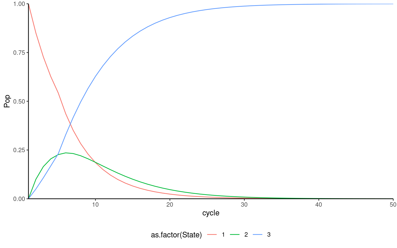
R
Not only is it orders of magnitude faster to use Reduce compared to for in R (for multiple nested calculations), it also results in more intuitive and less taxing code to read. The only thing to understand is that PrevCycle is an object, whilst ThisCycle is an index. For this reason, it is very important to name these objects in a way that can be easily understood by someone reviewing from the outside. For example, would the above code be easier or harder to understand if PrevCycle was just called x and ThisCycle was just called y? Now, imagine that instead of a simple if, the contents of the functional environment consisted of all of the different per-cycle calculations required inside of a cost-effectiveness model, perhaps 50+ calls to different user-defined functions, each of which calculating one column in the patient flow. The importance of intuitive naming increases as a model becomes more complicated to avoid having to continually rely on deduction to establish what is happening in the code. This is especially importance with Reduce, which will more often than not be used in multiple places throughout a cost-effectiveness model implemented in R.
For more top line processes like making nice tables out of model results, being highly efficient tends to be less important. Most of the effort on this front should be directed at the heavy lifting, like generation of patient flow sheets, extrapolation of clinical outcomes, and repetitive analyses like Probabilistic Sensitivity Analysis (Section 1.7.1), One-Way- and Two-Way-Sensitivity Analysis and Value of Information (Section 1.8).
14.4.6 UI Layouts conducive to cost-effectiveness models
Dashboards
We have found that so-called “dashboards” are very conducive to the presentation of economic models. Dashboards contain a strip on the left-hand side which can be minimised and provide links to several different pages for quick navigation through the model calculations, results and sensitivity analyses. Figure 14.2 provides an example of this structure.
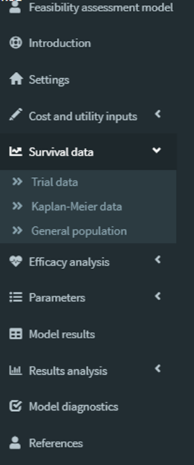
As can be seen, the tab-like interface is very familiar to those used to Excel-based models or web apps in general, albeit in a vertical rather than horizontal arrangement. The dashboard menu can be minimised to free up more of the screen space. Alternatively, it is possible to have the tabs as a menu in the bar at the top, but we have found that the extra click is often offputting for users.
Boxes and tabbed boxes
Boxes and tabbed boxes are excellent ways of directing the user’s attention towards something whilst maintaining a high level of clarity and transparency. Figure 14.3 and Figure 14.4 demonstrate the ability of a box to maintain a very simple and intuitive layout with clear signposting.
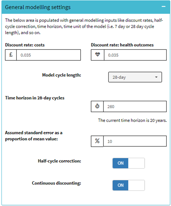
It is clear that the box contains general modelling settings like discount rates, cycle length, time horizon and so on. This box can also be minimised once the settings are entered, which is convenient as these settings are only likely to change in sensitivity analyses once determined.
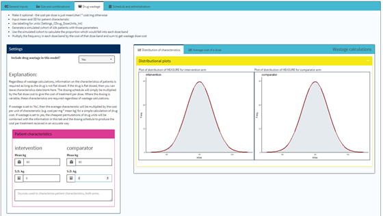
There are many inputs required to capture drug costs in a model. A tabbed box is convenient when it is desirable to collect them together, or to lead the user through a process using the tabs from left to right. In the example above, the user is led through a series of steps required to establish a schedule of costs and dosing. For example:
- General drug inputs: number (up to a reasonable maximum) and type (flat dosing, exact dosing based on patient characteristics, dose banding based on patient characteristics)
- Size and combinations: Number and size of available units in mg, mL etc
- Dosing: licensed dosing, relative dose intensity and so on
- Scheduling: loading dosing, frequency of dosing, dose breaks, time-based stopping rules
- Cost: List prices, discounts, other factors
- Allocation: Assignment of drugs to arms and model health states
- Preview: A summary of the final dosing schedule in units consumed and associated cost
All of these could be tabs, which lead the user through a journey of defining the drugs of interest to a cost-effectiveness evaluation. This is a lot of information, and to put all of this in one page implies a lot of scrolling, which could lead to steps being omitted. It is much more intuitive to go through the steps via tabs from left to right, filling in the required inputs in order.
Rhandsontables
Sometimes, there is just no substitute for an Excel-like table containing some data which is to then be used in model calculations. Fortunately another package rhansontable allows R/shiny to access a javascript package which can allow such tables to be used inside of a shiny application as an input/output mechanism for data. We recommend using these for instances in which the number of inputs (i.e. rows/columns) is unknown, or it visually makes sense for the inputs to be entered in an Excel-like way. Alternative methods do exist, which use renderUI to generate multiple separate numerical or other inputs iteratively.
Containers
Each element within the UI has a container of some kind around it. Each of these containers has its own features and behaviour, from expanding vertically to accommodate the contents and pushing the contents in the next row downward (i.e. a fluidRow), to a floating element which follows the user’s mouse pointer.
14.4.7 Deployment and security
When proposing the use of R and shiny to our clients in a professional setting, we have found the issue of deployment and security to be a point of major concern. Many clients are worried about exposure of source code, and having to interact with it in order to run the application locally. Others have expressed concern over remote hosting of the application and the security concerns that come with this. Protection of confidential discounts and patient level data are of particular concern.
These are all legitimate concerns. The best way to address the concern of sensitive data being accidentally released is to keep confidential inputs separate from the code. For example an inputs file containing sensitive discounts could be hosted on a secure server with only those who need access allowed it with the Shiny application having a button to upload the data. It is also possible to send the model to the data, rather than inputting the data into the model, using APIs.
If protection of code, rather than inputs, is required investment will be required in establishment of the correct infrastructure to ensure that any sensitive data is always protected, and the possibility of unauthorised access to the application is eliminated. This results in an application that is more secure than current practice (sending Excel files back and forth).
Rstudio Connect and shinyapps.io can be used to set up a platform for users to log into and use the application without having direct access to the source code. These are both products from Rstudio.
Rstudio Connect is a service which can be set up on a server of the user’s choosing, whereas shinyapps.io uses servers owned by Posit, the new incarnation of Rstudio developers. Consequently, Rstudio Connect is a more appealing choice in HEOR, due to its use of highly sensitive patient data and strict data control regulations.
Connect provides a full web user interface for the owner of the applications, in which they can act as an administrator of access and permissions to others. The application development process is still local until the point of “publication”, which results in an update of the remotely hosted version. This is analogous to performing updates on an Excel model and then emailing this updated version to a client, except a lot more secure, and without the need for sending emails containing large files
14.4.8 Workflow and version control
Workflow
The workflow when building a shiny application is different to that of building an Excel-based model. In Excel, the visual, the logical, and the computational all happen in the same place. When working with a shiny application this is not so. Instead:
- The generation and/or presentation of the visual happens in the UI script
- The logical, the computational, and some generation of the visual happen in the server script
Due to this, it is very important to remain organised (see Section 14.4.4). The importance of that organisation extends to the process of adding individual features. Working with code can make it tempting to “rabbit hole” by persisting with the creation of all sub-features of a feature until they work as intended. However, such a workflow makes it very difficult to maintain the overall structure of an application, as one does not have the same visual basis on which to organise one’s thoughts. Consequently, it is important to resist this temptation and organise the flow of work into defined and sequential blocks.
Typically, the workflow for building a new feature into a shiny application is as follows:
- An input or set of inputs are built into the UI (via the
uiscript, or viarenderUIin theserverscript anduiOutputin theuiscript) - Those inputs are processed and computed in the server, generating a set of reactive objects
- The outputs generated are either passed along the calculation chain into other reactive objects or fed into rendered outputs in
outputto be presented in the UI.
These steps are unconsciously familiar to any Excel user. A formula is placed in a cell linking to the results of preceding formulas and potentially some other data. That formula is evaluated, producing some results, which then feed into a graph, table, or further calculation. In this top-line sense, the workflow of shiny model development is strikingly similar to that of Excel.
When working with the reactiveValues list approach described in our tutorial in the online version of this book, this workflow is similar, but slightly different:
- An input or set of inputs are built into the UI (via the
uiscript, or viarenderUIin theserverscript anduiOutputin theuiscript) - A set of
observeEventevents are programmed to respond to changes in those UI inputs, cleaning and processing the data, then feeding the results into the organisedreactiveValueslist - Switches and triggers are programmed into the UI to feed the values from the organised
reactiveValueslist into its live version, which updates the UI presentation upon changing. - The lists are used in further calcualtions or converted into
outputelements to be presented in the UI.
There are a few exceptions to this flow. One such example is rhandsontable objects, which are generated as outputs in the server (via renderRHandsontable to create e.g. output$my_hot), and exist simultaneously as inputs (e.g. input$my_hot). In either approach the table is rendered, and its input equivalent is then used in the server under the same name. This is convenient for the reactiveValues list approach, as the entire table can simply be fed into the list R whenever it changes using the function hot_to_r. Simply set up a very simple observeEvent event. Note that you cannot just copy and paste the below and run it, and need to follow the instructions in the annotations.
# in the UI script, add the following 2 elements: the table and a confirm button

rhandsontable::rHandsontableOutput("my_hot")
shiny::actionButton("ui_commit_changes", "commit the changes to the table")

# In the global settings file, usually called global.R, generate the
# defaults inputs. This can also go in the main app.R file too, as long as it
# runs when the app runs to define the global environment beforehand.
# Alternatively, add it to the existing # D list.

D <- list(my_category = list(my_hot = mtcars))

# in the server, insert these elements. if `R` and L are already defined,
# put these elements in the desired location and amend the server code
# accordingly. Populating them here initially with some example data from core
# R. These values would normally come from object D, a list of default values
# for when the app first loads. To run this without shiny, simply run the
# following lines:
#
# R <- D
# L <- D
#
# and run through the lines inside of the shiny events

L <- shiny::reactiveValues(my_category = D$my_category)
R <- shiny::reactiveValues(my_category = D$my_category)

# Taking the "live" values L to populate the table, generate a hands on table:

output$my_hot <- rhandsontable::renderRHandsontable({
  dat <- L$my_category$my_hot
  rhandsontable::rhandsontable(dat)
})

# place the table in the "reactive" reactiveValues list R, only if it exists,
# immediately to keep a live record of the user inputs. Do this with a very
# high priority so that it happens before anything else. this avoids and
# flickering or looping.

shiny::observeEvent(input$my_hot, {
  req(!is.null(input$my_hot))
  dat <- rhandsontable::hot_to_r(input$my_hot)
  R$my_category$my_hot <- dat
}, priority = 100)

# when the user commits the changes feed them from `R` to L. As the hot
# values have already been converted back to `R` in the above, this is simply
# passing it along. Note how this links back to output$my_hot because
# L$my_category$my_hot has changed. This means that pressing the button may
# cause output$my_hot to refresh. Usually it does not because `R` = L once
# the button is pressed. Note that the priority of this event is even higher
# than the immediate watcher to force the update to be in line with R.

shiny::observeEvent(input$ui_commit_changes, {
  L$my_category$my_hot <- R$my_category$my_hot
}, priority = 101)

# That's it. Now whenever the user changes the table "my_hot", the server
# records those changes inside of `R` immediately. When the user presses the
# commit button, this moves the changes from `R` to L, meaning that if the
# table goes in and out of existence, its values will be preserved, similar to
# using isolate(). This simple system can be expanded to almost any level of
# complication.
#
# Finally, if an object S exists for a separately saved file, it can be
# loaded in to replace L and that will update the UI which will then update R.
# Loading from previous file would simply be L <- S, instead of thousands of
# lines of individual input updates!
So, with the more complicated workflows like the rhandsontable example, the workflow when working with central reactiveValues lists is actually simpler, as no renderUI is required inside of the server. The more typical workflow when using this system is as follows (for a set of individual numeric inputs, the number of which is unknown at runtime):
# For the UI, there are 3 inputs, how many numerics, the numeric inputs
# themselves, and the confirm button for L <- R. They are contained in 2
# objects, one containing all the inputs and one containing the button

shiny::uiOutput("ui_input_set")
shiny::uiOutput("ui_confirm_inputs")

# similar to the above in global, define the elements to enter into D

D <- list(my_category = list(
  n_inputs_max = 10,
  n_inputs     = 5,
  values       = 1:10
))

# pass these into `R` and L and set up the system, similarly to the above:

R <- shiny::reactiveValues(my_category = D$my_category)
L <- shiny::reactiveValues(my_category = D$my_category)

# generate a dynamic UI which responds to the amount of inputs the user wants.
# Note that this relies completely on L and not on `R` to avoid infinite
# looping!

output$ui_input_set <- shiny::renderUI({
  req(!is.null(L))

  # pull out the inputs for this category:

  LMC <- L$my_category

  # generate the n inputs input

  n_inputs <- numericInput(
    inputId = "ui_n_inputs",
    label   = "Select number of inputs required",
    max     = LMC$n_inputs_max,
    value   = LMC$n_inputs
  )

  # use those inputs to generate a list of numeric inputs. note that
  # L is being used to populate all values, and L is always there, so these
  # inputs have "memory"!

  input_list <- tagList(lapply(1:LMC$n_inputs, function(i_input) {
    shiny::numericInput(
      inputId = paste0("ui_my_inputs",i_input),
      label = paste0("ui_my_inputs",i_input),
      value = LMC$values[i_input],
      min = 0,
      width = "100%"
    )
  }))

  # put the individual bits above together into one thing:

  fluidRow(
    width = 12,
    column(
      12,
      n_inputs,
      hr(),
      input_list
    )
  )

})

# next we need to update `R` accordingly following changes to n, or the inputs:

shiny::observeEvent(input$ui_n_inputs, {
  if(!is.null(input$ui_n_inputs)) {
    R$my_category$n_inputs <- input$ui_n_inputs
  }
}, priority = 100)

# now for all possible inputs, trigger an event for that input which if that
# input exists passes its value to the appropriate place in R:

lapply(1:D$my_category$n_inputs_max, function(i_input) {

  # so, for this input paste0("ui_my_inputs",i_input) e.g. input$ui_my_inputs1,
  # if the value is not null (i.e. it exists, then get that value and pass it
  # to the reactive object R)

  observeEvent(input[[paste0("ui_my_inputs",i_input)]], {
    # require that the value exists (is not null), and then pass the value to R
    req(!is.null(input[[paste0("ui_my_inputs",i_input)]]))
    R$my_category$values[i_input] <- input[[paste0("ui_my_inputs",i_input)]]
  }, priority = 100)
})

# now we are updating `R` live we need a trigger to pass it to L when the
# button is pressed.

observeEvent(input$ui_confirm_inputs, {
  L$my_category <- R$my_category
}, priority = 101)

# Now, the user changes the number of inputs ui_n_inputs and this initially does
# nothing in the UI. when the user presses ui_confirm_inputs the number of
# inputs in the UI will then change. changing the individual inputs whilst
# the number of them is "out of date" will still work because they are always
# recorded in `R` immediately, so the app will remember everything (except for
# empty values as they will be ignored, which gets around a major issue with
# numericInput more generally in Shiny). Even those inputs that fall out of
# existence will be remembered (e.g.reduce ui_n_inputs, confirm, increase
# again, confirm. inputs should still "remember" their values)
So, regardless of the complication of the process, a user input is generated which is informed by L. Changes to that interface change R but not L, and a button updates L using R. The workflow for writing features using this approach is as follows:
- Add the structure and default values for the data to
Dso that there is data to populate the UI element with. Make sure that this includes any minima or maxima in dynamic contexts so that the user doesn’t have the choice to define large numbers of inputs (see above). - Feed the default values/structure into
RandLin the server. The values inLwill eventually feed intoRanyway, so this is a good test to run. - Build the user interface for entering values using
renderUIand popualte the UI elements only usingL(never hard-code or useR). Do not forget to build in a way for the user to updateLusing the values inR - Build the triggers to update
Rwhenever the user changes something in the associated UI elements. Iteration and using the defined maxima inDare both useful approaches here which can reduce lines of code considerably - Build the triggers to update
Lto be in line withR. This can and usually will be a button. However, other triggers are possible, like for example in the above, changinginput$ui_n_inputscould trigger the update ofR, and then immediately triggerL <- Rto streamline the process (see the example below). Alternatively, if in a tabbed environment liketabsetPanel, changing tab can trigger a simpleL <- Revent, if an id is provided in theidargument.
# one event to respond to changes in number of inputs, and then pass those
# changes to L immediately, triggering a refresh.

observeEvent(input$ui_n_inputs, {
  req(!is.null(input$ui_n_inputs))

  R$my_category$n_inputs <- input$ui_n_inputs
  L$my_category <- R$my_category

}, priority = 102)
The workflow for building shiny applications is essential to working efficiently and effectively. The above examples should provide some guidance as to good ways of working whilst keeping things organised and easily reviewed.
Version control
In-depth discussion of version control is provided in the well known freely available texts around the matter. (Chacon and Straub, 2014) We will therefore not repeat these arguments here. However, from a HEOR standpoint and given our experience working with and without version control on live R-based industry work, we would strongly recommend that it is used ubiquitously for R-based cost-effectiveness modelling, and for statistical analysis too.
Without version-control, we have found projects to be chaotic. Files are lost, people have to waste a large portion of their thinking on memorizing where things are, which file name to track and who is working on what aspect of the project. As version control standardises and controls all of this, it allows us to focus on our specalisms rather than file administration, whilst also preventing disasterous moments (for instance an excel model becoming corrupt without the ability to revert it to a previous version).
We have found collaboration with those initially completely new to (git style) version control to be initially slow-going as they learn, and to typically include some one-to-one tutoring sessions to get a basic understanding of the concept. However, once the basics and good practices are established, the improvements in efficiency and productivity have more than made up for the initial difficulties. We have found it to be very important to establish the workflow with those new to version control. In particular, we have found that the idea of making a branch of a project to build a feature and then submitting a pull request to allow the supervisor/leader review/QC those changes before allowing them into the main branch of code is alien to most at first. We recommend running through practical examples of this before allocating important work.
Overall, our advice for bringing those new to (in our case git) version control up to speed includes covering the following:
- Start with basic tutoring, including going through the steps of using
Rstudiowithgit, including- Making a repository on
GitHuborGitLab - Cloning said repository onto a local machine using the interface within
Rstudio - Making some changes and committing them, with instruction on frequency of committing
- Pushing the changes to the
gitrepository online - Refreshing the page on the website to see that the version has been updated
- Allowing some time for the student to do this repeatedly
- Making a repository on
- Instructions on workflows when collaborating
- Coaching on branching structure, and never just pushing changes to the
mainbranch - Pull requests and issues. The usefulness of a recorded discussion on each issue
- Practical work. Make a branch, make some changes in commits, submit pull request.
- Coaching on recursive branching, branching from a branch
- Coaching on branching structure, and never just pushing changes to the
Once someone has a grasp on this, they should then be in a position to build up their knowledge of working with version control, which will allow them to become more efficient.
Version control and shiny applications
In the past, we have typically worked with small focused teams on projects to create cost-effectiveness models in R with or without shiny. These have usually consisted of a strategic advisor, a technical lead, a technical team member and perhaps a statistician. The strategic advisor’s role is normally to oversee, and they do not need to review all changes as they happen. Consequently, the technical lead is usually the one responsible for the git repository. The repository is set up so that nobody can push changes directly to the main branch. This intentional limitation prevents erroneous code from replacing the current working version of the e.g. cost-effectiveness model, and means that all code that supersedes the current version must be QC’d before it is allowed to do so. Thus, the git workflow almost always follows the same pattern:
- A developer has an idea for or is instructed to build a model feature (e.g. drug wastage or EVPI)
- The developer makes a branch with a descriptive name (e.g.
drug_wastage, orevpi) - The developer then builds this code into the model, committing frequently and without having to worry about breaking anything, as the
mainbranch is unaltered - The developer eventually is satisfied that the feature is working properly and is creating correct results. The developer submits a pull request, to merge the changes they have made into the
mainbranch, pushing their changes to their branch - The whole development team, or specific members designated by the developer QC this additional code. As it is a branch, they can simply
pullthe changes to their own computers, switch to the branch and test the code themselves. They can also make corrections,committhem andpushthem, which will update the pull request code for the other reviewers topull. - Once the team is happy with the code in the pull request, they can approve it, which will merge the changes with the
mainbranch, updating the version of the model.
One new concept for many HTA modellers is the idea that any number of individual developers can follow the 6 steps above simultaneously, meaning that there is no limit to parallel working on a cost-effectiveness model. This has more recently become possible in Excel via Excel online, which allows multiple people to be working on an Excel file in SharePoint at the same time. Yet this has its issues as one has to endure simultaneous changes happening in real time (e.g. rows, columns, sheets, tables being added/removed whilst you were working on them), which can be distracting, or can even lead to errors which cannot be undone. In a git controlled world, developers are working on separate clones of the repository, so this is not an issue. Further, in a git controlled world, each developer is free to make mistakes without it permanently saving those mistakes into the one central file. There is a full history of all changes committed by all individuals, meaning changes can be reverted easily. git is used for large projects with literally thousands of developers working simultaneously on different features all at the same time, all within the same repository. In an industry which typically has very short development timelines for cost-effectiveness models, this could be extremely valuable, allowing more people to be allocated to development simultaneously with smaller loss of incremental productivity per team member added.
In our experience, well structured shiny applications are usually broken down into lots of files. This is conducive to version control as it avoids something called merge conflicts. These occur when two developers have changed the same lines of code in their separate workstreams. For instance, if one person is working on drug wastage and another on scheduling drug costs over time, then they might collide on something like loading dosing or weaning. If the code is well structured and separated out into files, they are likely to be working in different spaces to make these changes, and it is less likely that they will collide. However, this example highlights the importance of communication whilst also showing the power of git. One can simply attempt to merge the changes from one branch to the other to see if they collide (pull and then merge), and the resolution of any issues can then be proposed from one to the other via pull request. This formalises the issue, provides a basis for productive discussion, and allows the more senior team members to step in, review the code and proposed solution, amend and approve that solution and continue with the development of the model. This flexibility is extremely useful and efficient when working quickly under tight timelines, as the two developers can move onto different tasks whilst the leader resolves their issues, and finalises both features (or passes them back). No time is wasted and the entire team can work without interruption.
Much more detail than we could hope to include here is provided in Chacon and Straub (2014). We recommend that anyone working with git should at least read the early sections, and should refer to this book whenever they are stuck.
14.5 Conclusion
The use of shiny facilitates R model accessibility through the construction of interactive web applications which technical and non-technical stakeholders can interact with. This is why there is increasing interest in use within both industry and HTA bodies. The key to construction of user and reviewer-friendly shiny apps lies within the use of an appropriate project framework to organise code, good naming conventions, devotion of time to understanding user requirements and how these can be addressed using UI layout options, consideration of deployment options and security requirements early on in the project process and good workflow and version control. We look forward to seeing yourshiny apps in future!