# Defining the trajectory
traj <- trajectory() %>%

  # Nurse determines whether doctor should be visited
  seize(resource = 'Nurse') %>%
  timeout(task = function() rweibull(n = 1, shape = 5, scale = 10)) %>%
  set_attribute(
    keys = 'SeeDoctor', values = function() rbinom(n = 1, size = 1, prob = 0.3)
  ) %>%
  release(resource = 'Nurse') %>%

  # Only those who need to go through to the Doctor
  branch(
    option = function() get_attribute(.env = sim, keys = 'SeeDoctor'),
    continue = T,
    # Sub-trajectory for the doctor
    trajectory() %>%
      seize(resource = 'Doctor') %>%
      timeout(task = function() rweibull(n = 1, shape = 5, scale = 10)) %>%
      release(resource = 'Doctor')
  ) %>%

  # Some patients will have to be re-examined by the Nurse
  simmer::rollback(
    target = 5, check = function() rbinom(n = 1, size = 1, prob = 0.05)
  )

# Plots a diagram with the trajectory
plot(traj)


# Defining the simulation environment
sim <- simmer() %>%
  add_generator(
    name_prefix = 'Patient ',
    trajectory = traj,
    distribution = function() rexp(n = 1, rate = 0.1),
    mon = 2
  ) %>%
  add_resource(name = 'Nurse', capacity = 2) %>%
  add_resource(name = 'Doctor', capacity = 1)


# Running the simulation
set.seed(123)
sim %>% reset() %>% run(until = 4 * 60)


# Extracting the outcomes
df_arrivals <- get_mon_arrivals(sim)
df_resources <- get_mon_resources(sim)
df_attributes <- get_mon_attributes(sim)

# how many visits to the doctor's office?
df_attributes%>%
  filter(key=="SeeDoctor") %>%
  summarize(sum(value==1))

# Can visualise the first few rows of the resulting simulations
head(df_arrivals)
head(df_resources)
head(df_attributes)12 Discrete Event Simulation in R
Koen Degeling
GSK, Amersfoort, The Netherlands1
Mark Clements
Karolinska Institutet, Stockholm, Sweden
Erik Koffijberg
TechMed Centre, University of Twente, Enschede, The Netherlands
James O’ Mahony
University College Dublin, School of Economics, Dublin, Ireland
Mohsen Sadatsafavi
University of British Columbia, Vancouver, Canada
Petros Pechlivanoglou
The Hospital for Sick Children and University of Toronto, Toronto Canada
12.1 Introduction to Discrete Event Simulation
Discrete event simulation (DES) is a form of modeling that addresses the occurrence of discrete events and the leaps in time between them (Karnon and Haji Ali Afzali, 2014). It contrasts with discrete-time state transition models (DT-STMs) in how it defines state membership and how time progresses in the model. While DT-STMs such as (semi) Markov models have been popular in health economics and remain very common, DES has a number of important advantages and seems a likely candidate for increased adoption. Specifically, by its handling of time and given its modelling of individual level trajectories, DES makes it easier to incorporate detailed clinical data, especially time-to-event data, to model complex clinical care pathways, and evaluate personalised interventions compared to DT-STM. In some settings it can also provide significant computational advantade over DT-STMs.
This introduction first considers some of the characteristics of DES. It then describes some of the advantages of the DES approach as applied to health economic decision modelling. The particular context assumed here is the economic evaluation of healthcare interventions.
12.1.1 What is DES?
DES is the modelling of a system as it changes with time by representing the instantaneous occurrences of events at separate points in time (Law and Kelton., 2007). Karnon and Haji Ali Afzali (2014) provide a clear conceptual overview of DES in its application to healthcare modelling. They note that DES models can be applied with and without explicit capacity constraints on the resources used in the model. Those with resource constraints might include scarce clinician availability on a hospital ward and typically involve the simulation of patient queuing systems including triage by severity of need. Examples of such DES applications include the optimization of surgical services and intensive care unit care capacity (Stahl et al., 2004; Wullink et al., 2007). Those without explicit capacity constraints might correspond more broadly to the type of health economic analyses in which overall resource scarcity is proxied by a cost-effectiveness threshold. While DES is particularly useful for the simulation of the former type of analyses, they can also be useful for the more general health economic modelling applications. Examples of DES applications without capacity constraints can be found in analyses of smoking cessation interventions, cancer therapy and treatment for schizophrenia (Degeling et al., 2024; Dilla et al., 2014; Xenakis et al., 2011). In this chapter we will mainly focus on the latter type, but we will briefly provide guidance on how one can address capacity constraints using R.
Karnon and Haji Ali Afzali (2014) describe six core concepts in DES of entities, attributes, events, timing, resources and queues. The final two concepts of resources and queues are less relevant to health economic analyses without explicit capacity constraints, but the preceding four remain essential. Below we describe each concept in more detail:
DES is inherently an individual-level simulation (or microsimulation) approach in which individual entities are modelled. This contrasts with the cohort-based simulation approach commonly applied in DT-STMs, in which a group of simulated patients typically start in one health state and are then distributed over a number of other states over time as time progresses.
A typical DES model will simulate the time between a series of events for each simulated entity. These events may be sequential, or related, in that one event logically follows another. Their ordering may also be stochastic in that they may be determined by sampling from joint distributions. Events may also be repeating in that a given series of events may reoccur, or can be competing, in that the occurrence of one event can prevent an entity from experiencing another event. For example, death from cancer may compete with death from another cause.
The timing of events will typically be simulated as a stochastic process. For example, the time to disease onset will likely be modeled as a random variable. Conversely, the timing of other processes may be deterministic, such as the sequencing of episodes of care which may occur on a predictable basis, such as monthly transfusions. The simulation of stochastic events will typically be implemented by drawing from specified probability distributions for the particular time-to-event using pseudorandom number generators. The timing of events may also be correlated with other distributions in the model to simulate associations between the probabilities of different events, or their consequences in terms of impact on health and costs.
These distributions may vary between individuals in the model according to attributes of the simulated entities. These attributes may be those known at the outset of the simulation, such as age and sex, or they may be determined within the model, possibly in response to the progression of a continuous process such as disease development or in response to discrete events such as treatment success or failure (Caro and Ishak, 2010).
The popularity of discrete time approaches to date may in part be due to the fact that DT-STMs can be easily implemented in readily available spreadsheet software (Menn and Holle, 2009). Accordingly, software availability and basic simulation skills have not been a meaningful barrier. Although there are examples of DES implemented in common spreadsheet software (Gestel et al., 2010; Griffiths et al., 2010), most DES approaches have either relied on proprietary software or required at least a modest degree of programming skill to build. There is growing popularity of the R programming language for health economic modelling and the increasing array of resources supporting modelling (Jalal et al., 2017), means the prospects for increased use of DES appear strong.
12.1.2 Existing DES resources in R
While DES is an established simulation method, previous authors have noted implementations in R have been relatively few (Lawson and Leemis, 2015). The DES package is a relatively simple package with limited dependencies in R (Matloff, 2017). The most notable DES package in R may be simmer, which has the ability to simulate capacity constrained systems and incorporates C++ code to improve processing speed (Ucar et al., 2019). The descem package permits cost-effectiveness analysis using both DES and Markov approaches in contexts without capacity constraints (Aponte Ribero and Sanchez Alvarez, 2022). It is a recent development and not yet optimised for efficient run time and the present emphasis is on transparency. Other packages with DES capabilities include the packages gems (Blaser et al., 2015) and flexsurv (Jackson, 2016) which both allow for the development of DES models without resource constraints.
12.1.3 Advantages of DES
As a microsimulation approach, DES naturally permits retaining information on attributes of each entity and thus avoiding problems resulting from the the memory-less property of cohort state transition models and the cumbersome workarounds required to avoid this property. Similarly, DES is also better suited to the simulation of processes with time-varying event rates (Karnon and Haji Ali Afzali, 2014). The simulation of such time-varying rates can be important for the accurate simulation of disease processes which include non-constant hazards rates. A closely related consideration is that event rates can be contingent on prior events. Discrete event simulation is well suited for recording previous health events for simulated individuals. Rates that vary with prior disease history can be relatively easily implemented in a DES that records prior health events. Other advantages is that DES is better suited to model calibration and to incorporate data that include heterogeneous patient populations and the subsequent simulation of such heterogeneous populations (Karnon and Haji Ali Afzali, 2014).
DES mdels do not require the assignment of individuals in mutually exclusive health states (Standfield et al., 2014). This brings the advantage of parsimony to a model, as it does not require proliferation of health states to simulate multiple potential co-occurring situations. It may also bring the benefit of flexibility as events and states can be added or subtracted from a model without requiring large changes to the model structure. For example, the influence of a co-morbid state on disease progression and treatment outcomes could be added to a model without having to replicate the prior model structure in order to simulate patients with and without the specific comorbidity. The existing model structure can be retained and the influence of the co-morbidity can be captured by applying relevant parameter adjustments.
As opposed to discrete-time simulation approaches, DES models handle time continuously hence there is no loss of accuracy due to the discrete approximation of inherently continuous processes. DES also avoid the problems of multiple events potentially coinciding within a single discrete-time interval, when in reality they would occur sequentially. Continuous-time modelling not only avoids the discretisation of time, but also allows for modeling continuous disease processes, permitting more representative simulation (Karnon and Haji Ali Afzali, 2014). Continuous-time approaches are likely better suited to parameterisation against data that is typically recorded on a continuous time-to-event basis, though some data may of course be recorded at discrete intervals.
A DES may have advantages of computational efficiency as events only happen computationally when they occur in the model (Karnon and Haji Ali Afzali, 2014). By contrast, in a discrete-time microsimulation, even when no events happen, the simulation still needs to compute each new discrete interval, assign a transition probability and sample whether the event occured or not, even though state membership may not change in the new period. The computational advantage of DES in this respect will increase relative to a discrete approach as the interval length within the discrete approach is shortened as to reduce the errors due to discrete approximation, or similarly when events are relatively sparse and far from eachother in the time scale.
DES has been described as an intuitive modelling approach (Karnon and Haji Ali Afzali, 2014). The analyst conceives of the simulation problem in terms of the sequence of events and the length of time in between. This may be more intuitive than conceiving most inherently continuous processes in a discrete time framework in which state membership is updated over arbitrary time cycles.
12.1.4 Disadvantages of DES
A DES may be more time-consuming than conventional cohort-based discrete time approaches for analysts to code and for regulators to review (Karnon and Haji Ali Afzali, 2014), though this may primarily be a consequence of current relative lack of familiarity with DES rather than any inherent greater degree of complexity. Accordingly, HTA lacks an established common technical basis for DES simulation. This means DES models may lack transparency, as any analyst must be versed in the particular programming language any given implementation is coded in, including any particular packages employed. This barrier to transparency appears an important impediment to the acceptance and broader proliferation of DES in HTA.
12.1.5 Examples of DES in health economic analyses
Below we provide a non exhaustive review of DES in health economic analysis. Jun et al. (1999) provide an early survey of the use of DES in healthcare, while Zhang (2018) provides a more recent analysis. Both studies find that the majority of applications relate to patient flow and the allocation of scarce clinical capacity rather than health economic evaluation. Campbell et al. (2001) provide an early example of DES applied to a cost-minimisation analysis of home versus inpatient care for elderly care using the Simul8 software. Karnon and Haji Ali Afzali (2014) compares a spreadsheet-based Markov simulation of alternative breast cancer therapies to a DES implemented using the Crystalball software to compare run time and simulation accuracy. Similarly, Simpson et al. (2009) compare the Markov and DES modelling approaches using the Arena® software. Degeling et al. (2018a) conducted a similar comparison study in the context of colorectal cancer therapy using the Anylogic software. DES has also been applied to cancer screening, including implementations in Arena® and MS Excel (Griffin et al., 2020)
12.2 Chapter boundaries
Two of the components that define a DES are entities, which often in an HTA setting refer to an individual, and available resources. We will use the term ‘individual’ to denote simulated hypothetical individuals, such as healthy individuals or patients. We will use the term ‘resources’ to indicate, for example, operating rooms, medical supplies, and healthcare professionals. Some simulations may explicitly model constrained resources by limiting the availability of such assets as they are (temporarily) used by individuals potentially blocking access to these resources by other individuals. The example in tgus chapter, however, does not cover resources and their use, since in standard health economic evaluations resource constraints are typically not included explicitly but accounted for implicitly through the use of a cost-effectiveness threshold.
While individuals in DES can potentially interact, in practice few DES actually implement such interactions. This is most likely due to the fact that any interaction between individuals would require defining a specific time for it to occur, while in the DES individuals typically experience events at their own unique times, that is, time to events is determined independently for all individuals. Conversely, in discrete-time models time intervals within which events may occur are identical for all individuals, making it easier to implement interactions. Although interactions may be implemented in discrete-time STMs, the use of agent-based models for this purpose is much more common, for example in the context of infectious disease models (Hunter and Kelleher, 2021; Naimark et al., 2021). Agent-based models allow specification of the behaviour of agents, and individuals are defined as a specific type of agent. In agent-based models the behaviour of agents can drive the interactions and their outcomes, with all interactions occurring at discrete time points. In this chapter we will therefore not include interactions between individuals but focus on the core advantages of DES.
Finally, as discussed in the introduction and above, DES shares many characteristics with other modelling paradigms. Here, we will focus foremost on aspects that are unique to DES. Consequently model parameterisation, model calibration, and sensitivity analysis will not be discussed. While certainly useful for DES, this information can be obtained from introductory textbooks on simulation modelling (Law and Kelton., 2007) or other chapters of this book. Since DES distinctively requires the definition of time-to-event distributions, how such distributions can be fitted based on concrete data will be briefly illustrated. Further discussion on survival modelling can be found in Chapter 7 of this book.
12.3 Methods of interest when applying DES
While the focus of this chapter is describing how DES can be implemented in R it also presents some more general methodological content to ensure those new to individual-level modelling are provided with sufficient contextual material. First, a brief overview of the different types and levels of variation and uncertainty in individual-level models will be provided. Second, different approaches towards implementing competing events in DES will be discussed. Finally, aspects specific to DES will be covered regarding discounting health and economic outcomes over time.
12.3.1 Variation and uncertainty in individual-level models
Individual-level modelling techniques permit examination of the impact of different types of variation and uncertainty on model outcomes: heterogeneity, stochastic uncertainty, parameter uncertainty, and structural uncertainty (Briggs et al., 2012). Although parameter and structural uncertainty also apply to cohort-level models, and those can be parameterised and analysed for population subgroups to indirectly account for heterogeneity, stochastic uncertainty is specific to individual-level models. Heterogeneity can be incorporated in individual level models e.g. through variation of baseline characteristics among simulated individuals. Clearly distinguishing between these different types of variation and uncertainty, and appropriately modelling them, is essential.
12.3.2 Heterogeneity
Heterogeneity, a well-known concept in health care and the medical literature, refers to the variability between individuals that is explained by individuals’ characteristics (Briggs et al., 2012). In cancer, for example, differences in outcomes between individuals may be explained by the disease stage at diagnosis or the presence or absence of a particular biomarker. The need to account for heterogeneity in health economic models is one of the main reasons to use individual-level modelling, as each hypothetical individual can be assigned certain characteristics that influence their disease pathway and outcomes in the model.
12.3.3 Stochastic uncertainty
Stochastic uncertainty, also referred to as first-order uncertainty, refers to random variability between identical individuals (Briggs et al., 2012). A common example of stochastic uncertainty in DES is drawing time-to-events from a parametric distribution, such as sampling time to cancer recurrence like in the case study. Even if the same time-to-event distribution is used for all individuals, their individual time-to-events will differ. Another common example of stochastic uncertainty in individual-level models is that simulated individuals may experience different events they are at risk of purely by chance. Stochastic uncertainty creates random variation in output estimates and sufficient simulated individuals are needed to ensure that the average outcomes have converged, i.e. stable model outcomes are obtained. Given that most decision models are nonlinear in nature, such stochastic variation is important to be captured even if the focus is on the expected value of the outcomes.
12.3.4 Comparing heterogeneity and stochastic uncertainty
Because both heterogeneity and stochastic uncertainty result in variation between individuals, it is important to clearly distinguish between the two. Consider the example of modelling time-to-recurrence based on patient and disease characteristics. One may first incorporate heterogeneity by varying the distribution scale parameter based on those characteristics and then draw a random time from that distribution. In this way, the resulting random draws contain a mix of individual level variation due to heterogeneity and stochastic uncertainty. Heterogeneity is present because different subgroups of patients will have different scale parameters for the time-to-event distribution, but stochastic uncertainty is also present because individuals with the same distribution parameters will still have different time-to-events that are sampled from it.
Frailty models are a more complex example. In such models, the distribution parameters may be different for subgroups of individuals, due to heterogeneity, but also due to chance for individuals with the same characteristics (i.e. stochastic uncertainty). Consequently, there may be heterogeneity and stochastic uncertainty in the value of the time-to-event distribution parameters, based on which a second layer of stochastic uncertainty is introduced by sampling from the resulting individual-specific distribution. This frailty component is not captured in this chapter.
12.3.5 Parameter uncertainty
Parameter uncertainty, also referred to as second-order uncertainty, refers to the uncertainty in the model parameters that arises from the fact that these are mostly estimated on a limited sample (Briggs et al., 2012). To illustrate the concept of parameter uncertainty, consider two randomised clinical trials that are performed in similar settings and with identical inclusion criteria, but with inherently different patient samples. Parameter uncertainty accounts for the fact that estimating a parameter value based on the datasets of these two trials may result in slightly different estimates. The impact of the parameter uncertainty on the uncertainty around model outcomes is typically examined through probabilistic analysis of the model. In such analyses, the model is evaluated for different parameter values sampled from distributions that define the uncertainty in the parameters. If the model is correctly specified and sufficient samples, i.e. model runs, are performed for the mean outcomes to converge, this mean is the only unbiased estimate of the outcomes of interest (Pieters et al., 2020).
12.3.6 Parameter uncertainty in individual-level models
The concept of accounting for parameter uncertainty in individual-level models is the same as for cohort-level models. Individual-level models, just like cohort models, often include parametric distributions. For example, a Gompertz distribution, defined by a shape and rate parameter, may be used to model background mortality. Given that these shape and rate parameters are typically highly correlated when the parameters of such a distribution are estimated from a sample, this correlation needs to be accounted for when sampling values for these parameters in the probabilistic analysis. When using a frequentist approach towards parameter estimation, two common approaches to account for the correlation between parameters of a distribution are using multivariate distributions or to use a non-parametric bootstrapping approach (Degeling et al., 2017). A benefit of the latter approach is that it can account for correlation between different distributions that are estimated based on a single dataset. When using a Bayesian approach towards parameter estimation, parameter values from the posterior distribution can be used to account for parameter uncertainty.
12.3.7 Structural uncertainty
Structural uncertainty, also referred to as model uncertainty, refers to the uncertainty in the model outcomes that arises from the assumptions that are made in the modelling process (Briggs et al., 2012). Examples of sources of structural uncertainty are, among other, the model structure and type of distributions used to model or extrapolate time-to-event data. In contrast with stochastic and parameter uncertainty, there is no gold standard for examining structural uncertainty. Although most studies exploring structural uncertainty have done so through scenario analyses in which outcomes are estimated under other assumptions, different approaches have been proposed, including model selection, model averaging, parameterisation of assumptions, and the discrepancy approach (Haji Ali Afzali and Karnon, 2015).
In summary, heterogeneity refers to variation between individuals that can be explained by their characteristics, stochastic uncertainty refers to variation between individuals that cannot be explained by their characteristics, parameter uncertainty refers to uncertainty in the estimated values for the parameters that define the model, and structural uncertainty refers to the uncertainty in model outcomes that arise from assumptions and decisions made in the modelling process. In the case study that is presented in this chapter, stochastic and parameter uncertainty are accounted for, but heterogeneity is only applicable in that outcomes differ between the two treatment strategies, whereas structural uncertainty is not explored.
12.3.8 Modelling competing events in DES
Competing events or risks are those that prevent other events from occurring, or change their likelihood of occurrence. Competing risks apply to the vast majority of health economic models as they represent different, competing, transitions to subsequent model states. As in the case study, common examples of competing events include disease recurrence or progression and death. Competing events are typically implemented in both cohort- and individual-level state-transition models using appropriately estimated transition probabilities for discrete time cycles, whereas DES provides enhanced flexibility to implement competing events.
If modellers have access to individual-level data, they have to select an approach towards implementing competing events in a DES. If only aggregate data are available, for example from published literature, the way in which those data have been analysed dictates how the competing events are to be implemented. Four general strategies for implementing competing events in DES have been identified: 1) simulating times for all competing events and selecting the event that is the first to occur, 2) sampling the event to occur first and the corresponding time-to-event second, 3) sampling the time-to-event first and the corresponding event second, and 4) using discretized cyclic probabilities to resemble discrete-time state-transition models, such as Markov models (Barton et al., 2004). These different strategies toward implementing competing risks do not only determine how events are simulated, but also how the data are to be analyzed.
A general recommendation has been made to use the third strategy of selecting the time first, based on a combined time-to-event distribution of all competing events, and subsequently selecting the event corresponding to that time, for example using a (multinomial) logistic regression model (Karnon et al., 2012). However, a simulation study for uncensored data emphasized the importance that such a single time-to-event distribution appropriately needs to model any multimodality in this distribution arising from difference in the time-to-events between events, for example using a mixture distribution of survival spline (Degeling et al., 2018b). This study also found an approach based on the second strategy, using event-specific probabilities to select the event first and subsequently select the time-to-event using event-specific distributions, had a similar performance but was more straightforward to implement. In case of censoring, however, this approach is not straightforward to implement and, depending on data characteristics, an approach based on the first or third strategy may be preferred (Degeling et al., 2022).
Besides the presence and level of censoring and other data characteristics, other aspects may influence the decision which approach towards implementing competing events is preferable. For example, if multivariable survival models are used to reflect heterogeneity or reflect for confounding in real-world data, the third strategy may be considered preferable by some because it only requires one survival model to be parametrized based on covariates. A discussion of such aspects is beyond the scope of this chapter, but it is important to be aware of the flexibility that DES provides. In the case study that will be presented later in this chapter, which is informed by censored data, an approach based on the first strategy is implemented.
12.3.9 Discounting in DES
Discounting is an integral part of health economic modelling and refers to the process of determining the present value of health and economic outcomes that occur in the future (Attema et al., 2018). Outcomes are typically discounted at discrete time intervals, such as in discrete-time state-transition models, but can also be discounted over a continuous period of time. DES allows either approach to be used. For example, treatment costs can be discounted at the time where they occur, but (quality-adjusted) life years can be discounted over a period of time. Equation 12.1 describes how one can discount a value (V) at a specific point in time \(t\) at a given discount rate \(r\) to obtain the net present value NPV. Similarly, the formula to discount a certain amount over a period of time from \(t_{\rm{start}}\) to \(t_{\rm{end}}\) to get the cumulative NPV (cNPV) is presented in Equation 12.2. While both discrete and continuous discounting can be applied to DES, the latter seems the more natural choice as state membership is not simulated over discrete intervals. Both these will be used in the case study to discount costs and effects, respectively.
\[\text{NPV} = \frac{\text{V}} {(1+r)^t} \tag{12.1}\]
\[\text{cNPV} = \int_{t_{\rm{start}}}^{t_{\rm{end}}} \frac{\text{V}} {(1+r)^x}dx \tag{12.2}\]
12.3.10 Decisions when implementing DES in R
Regarding model implementation, this chapter focuses on a process-based approach using the simmer package. Alternative approaches are also provided in an online appendix of this book, available at the website https://gianluca.statistica.it/books/online/r-hta/. This section considers the choices the modeller must make between these alternative implementations and what might motivate those decisions.
The model’s application will naturally inform which approach will be most suitable. Since models with relatively simple structures will be easier to construct and faster to run, the choice may not be so critical as the model should be transparent irrespective of what approach it is coded under. A model with many events will likely be slower to run and the analyst may need to choose an approach that is optimised for speed. This is especially a concern when considering the requirements for uncertainty analysis. The options for increasing speed include expanding the computing resources available, using parallel processing, using coding specific components in lower level languages such C++ or rely on packages such as simmer that use C++ as part of their functioning. Drawbacks of these approaches include the need for familiarity with C++ or simmer. Greater speed can also be achieved using a vectorised approach to microsimulation, which employs large arrays of simulated individuals and conducts operations on large numbers of entities simultaneously rather than one by one. However, vectorisation can be difficult to implement in complex model structures and the advantage of this approach may ultimately break down.
Transparency can be a relevant consideration in many cases. This may be both internal and external to the work environment the modelling is conducted in. The requirement to share models with those other than its builder means code and documentation should be accessible. Furthermore, the model may need to be read by external parties such as clients or regulators. Naturally this requires such parties to be both literate in R itself and willing to accept models coded in it, neither of which can be assumed. It also requires familiarity with the specific methods implemented. Reliance on packages also prompts blackbox concerns, and may result in version-specific issues, as the functioning and reliability of model components cannot be guaranteed by users. This may prompt modellers to opt for models that avoid heavy reliance on packages and more on R code. The trade-off here is that the code will likely be more voluminous as many functions must be coded from fundamental operations. Furthermore, coding from base R does not eliminate reliability concerns, as models still require validation.
The resources available to the modeler are a natural determinant of the choices available to them. High capacity computing power or networked access to powerful virtual machines may not be available to all modellers. In those instances, more efficient coding is required. As mentioned above, this itself requires coding experience.
12.3.11 Replicability in stochastic modeling
DES typically makes heavy use of random numbers to draw from parameter distributions. To ensure comparability between model runs which can be useful for demonstrating reproducability and assisting debugging it is useful to draw upon the same random numbers. The set.seed function in R permits reproducibility in the random numbers used between model iterations. It is important that any use of the set.seed function does not inhibit variation between iterations where it is required, such as between PSA iterations. In certain instances it may be necessary to record the random number draws on which model runs are based. The “bookkeeping” effort of writing and storing large arrays of random numbers can consume considerable computational resources and these will need to be considered.
12.4 Case study introduction
We illustrate the application of DES model in R through a case study on the cost-effectiveness of adjuvant therapy in colorectal cancer. The case study utilises the colon dataset that is freely available from the survival package. This dataset represents a randomised clinical study that was performed in the 1980s to investigate the efficacy of post-surgery adjuvant therapy for colon cancer. The trial included three arms:
- Observation (Obs), i.e. no treatment
- Levamisole (Lev)
- Levamisole and fluorouracil (Lev+5FU)
More information on the trial can be found in Moertel et al. (1990) and across other chapters of this book.
In our case study we performed a DES based cost-utility analysis and the primary source of input was the Moertel et al clinical trial. The DES we developed models individuals through cycles of treatment and multiple recurrence events and until death from cancer or non-cancer causes. The pathway of patients in the model is represented by the following high-level structure:
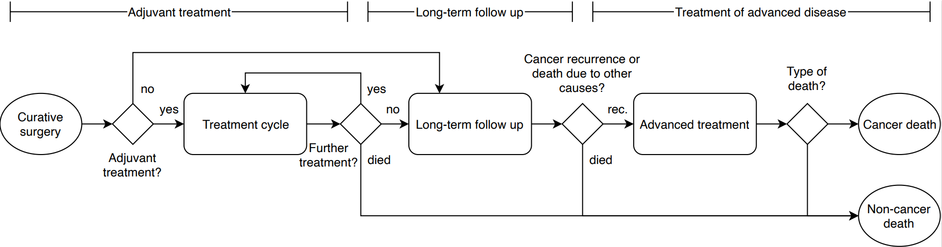
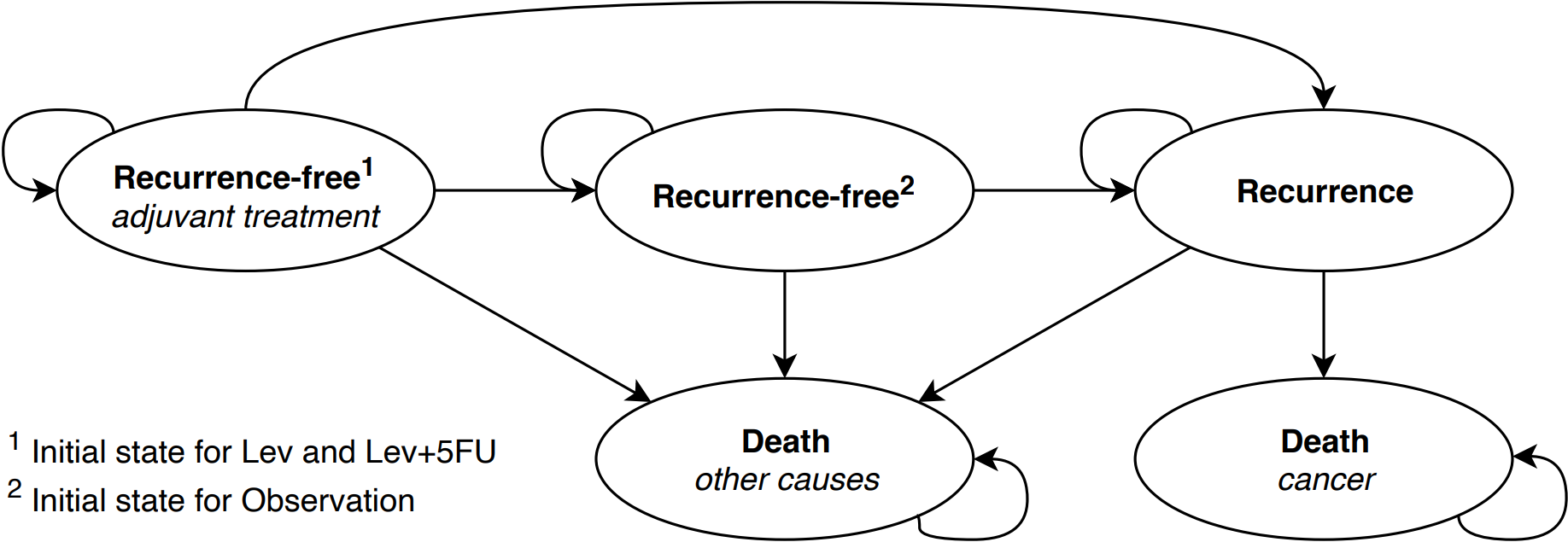
The natural pathway described above can also be more concisely presented through a model bubble diagram.
Events such a recurrence and death were assumed to occur in continuous time, while chemotherapy treatment was assumed to occur on discrete treatment cycles. A discount rate of 4% for costs and 1.5% for effects was assumed to illustrate the application of differential discounting, which aligns with the Dutch discount rate assumption. Discounting for costs was applied at the beginning of a treatment cycle.
12.4.1 Input parameters
Time to recurrence/ death
We estimated time to event for the modelled events using as input the colon dataset and applying a series of parametric survival models. We used best practice in model fitting and estimated a series of models including spline and mixture cure models. Details on model fitting can be found alongside the supplemental R code in GitHub and Chapter 7. We used US life-tables to inform the risk of death from other causes.
Costs and Utilities
Given the educational nature of this example, estimates for clinical input parameters, such as the probability of toxicities during adjuvant treatment, costs, and health utilities were assigned hypothetical values so that the outcomes present an interesting set of results. All distributions and parameters are presented in the Table below
| Parameter | Values | R variable name |
|---|---|---|
| Maximum number of adjuvant chemotherapy cycles | 10 | n_max_adjuvant_cycles |
| Length of adjuvant cycle in years | 3/52 | t_ adjuvant_cycle |
| Treatment Cost | ||
| Lev ($) | 5,000 | c_adjuvant_cycle_1 |
| Lev+5FU ($) | 10,000 | c_adjuvant_cycle_2 |
| Cost of toxicities ($) | 2,000 | c_tox |
| state costs | ||
| one time cost of recurrence ($) | 40,000 | c_advanced |
| Probability of toxicity per cycle | ||
| Lev | 0.2 | p_tox_1 |
| Lev+5FU | 0.4 | p_tox_2 |
| Health Utilities | ||
| Utility during adjuvant therapy | 0.7 | u_adjuvant |
| disutility associated with treatment toxicity | 0.1 | u_dis_tox |
| Utility when recurrence free | 0.8 | u_diseasefree |
| Utility after recurrence | 0.6 | u_advanced |
Adjuvant treatments and toxicities
Adjuvant treatments (Lev and Lev+5FU) are assumed for a maximum of 10 cycles and last for 3 weeks. Toxicities may occur during an adjuvant treatment cycle with a given probability that is different for each treatment (see Table above). There is no maximum on the number of toxicities that a patient can experience, with a maximum of 1 per treatment cycle.
We assumed that health utility during adjuvant therapy and during recurrence do not differ between treatments. Similarly the disutility of toxicities was not different between treatments and was applied to the complete cycle in which a patient experiences a toxicity. Quality-adjusted life-years (QALYs) are obtained by discounting and integrating utility over the duration of the cycle. During long-term follow up a constant health utility was assumed.
Treatment of recurrence/advanced disease
Individuals experiencing recurrence incur a one-time cost that was assumed to be independent of the treatment arm.
12.4.2 Implementation of DES in R
In this Chapter we provide four alternative ways of implementing a DES in R. We present two approaches in the main chapter and offer two more in the online appendix (https://gianluca.statistica.it/books/online/r-hta/). We also provide strengths and weaknesses for each implementation below.
12.4.3 Discrete event simulation in R using simmer
There are several options for implementing a discrete event simulation (DES) in R. A process-based approach is provided by the simmer package. Before diving into the code, a high-level introduction to the simmer package and some of its most fundamental functions will be provided. More information on the simmer package and on additional functions such as those to take into account resources and capacity constraints, can be found using the help function in R Studio, in related publications (Ucar et al., 2017), or its website https://r-simmer.org/.
When implementing a DES using simmer, two objects need to be defined: the trajectory and the simulation environment.
The Trajectory
The trajectory defines the structure of the model and, thereby what may happen to the simulated individuals. Therefore, trajectories define what events the simulated individuals may experience and what actions are performed. They are defined using the trajectory() function, which defines an empty trajectory that can be expanded using different building blocks.
Five fundamental building blocks for defining trajectories are:
- Attributes are used to store numerical information on an individual or global level. For example, attributes can be used to store characteristics (e.g., disease stage), outcomes (e.g., accumulated quality-adjusted life years and costs), and individualized model parameters and settings (e.g., sampled time-to-events or risk predictions based on characteristics and intermediate outcomes). Individual- and global-level attributes can be defined or updated using the
set_attribute()andset_global()functions, and read using theget_attribute()andget_global()functions, respectively. - Timeouts or delays are used to control the duration of time between different events or actions. In other words, it is used to set the time to the next event in the pathway, which generally is referred to as a time-to-event. An individual can be delayed for a certain amount of time using the
timeout()function or using thetimeout_from_attribute()if the duration of the delay is saved in an attribute. - Resources are objects that are shared between agents and which may have limited capacity. Example of capacity-constrained resources in health care may include the number of nurses in a particular department, the number of operating rooms, or the number of times a particular device can be used on a given day, such as a computerized tomography scanner. Resources can be occupied using the
seize()function, and they can subsequently be made available to other agents in the simulation using therelease()function. As explained in the Case Study Introduction, resources are not considered in the example, but their use is explained here regardless because the potential to implement resources is an important differentiator of DES. - Branches are used to allocate individuals to different sub-trajectories, i.e. to fork the trajectory. For example, branches may be used to implement competing risks, such as continuing to the next treatment cycle vs. stopping treatment, or being admitted as an inpatient from the emergency department vs. being discharged, where the sub-trajectories within the branch correspond to the competing events. The
branch()function can be used to implement a branch, where sub-trajectories can be defined within the branch, or individuals can skip the branch to continue in the main trajectory. - Rollbacks move an individual a number of steps back in the trajectory and can be used to repeat sections of the trajectory, which is useful for modeling repetitive activities such as treatment cycles. Rollbacks are implemented using the
rollback()function.
Other potentially useful trajectory-related functions are the functions join() to combine or refer to trajectory objects, log_() to log messages to the console for model building and debugging, and plot() from the simmer.plot package to plot a trajectory. The user should be reminded that some function names might be competing with functions from different packages.
The simulation environment
The simulation environment defines how many individuals enter the trajectory and when they enter, as well as what information should be gathered about the individuals and the resources throughout the simulation. Simulations environments are defined using the simmer() function, which defines an empty environment that can be expanded using different building blocks:
- Generators define the cohort of agents that will be simulated. The
add_generator()function can be used to define a cohort of particular individuals (also referred to as agents), which trajectory they should enter, and when that should be. - Resources define the amount and schedule of a type of resource to be available in the simulation. This can be defined using the
add_resource()function. These resources correspond to those used in the trajectory, such as professional staff and equipment in a health care setting. - Simulations can be performed using the
run()function, where thereset()function is useful to reset the simulation environment to its initial state. - Outcomes are saved in the simulation environment and can be extracted using the
get_mon_arrivals(),get_mon_attributes(), andget_mon_resources()functions, which return long-formatdata.frameswith a complete log of how values have changed throughout the simulation. The monitoring of arrivals provides information on when the simulated entities entered the simulation, when they completed the simulation, and how much time of the simulation they spend on activities rather than waiting in queues. The monitoring of attributes provides information on what attributes were defined or updated for each entity, including information on when the attribute was defined/updated and what the corresponding value was. The monitoring of resources provides information about how the utilization and queue for each resource changed throughout the simulation.
Use of these functions is illustrated below through a basic example that implements the process of a individual visiting a doctor’s office:
- When the Individual (agent) arrives to the doctor’s office, two Nurses (resource) are available to determine whether the individual needs to see the Doctor.
- The duration that they spent with the Nurse until it is determined if the individual needs to see the Doctor is sampled from a Weibull distribution.
- Whether the Patient needs to see the Doctor (resource) is stored in a ‘SeeDoctor’ attribute (1 = yes, 0 = no), which is performed during the Nurse visit.
- The probability that a Patient needs to see the Doctor is 0.3, which is used to sample the value for the ‘SeeDoctor’ attribute (1 = yes, 0 = no) and the time that the examination takes is sampled from a Weibull distribution.
- Based on the ‘SeeDoctor’ attribute, the branch directs Patient to the Doctor (sub-trajectory 1 , SeeDoctor = 1) or not (skip branch, SeeDoctor = 0). This branch is clearly visible when the trajectory is plotted using the
plot()function, as demonstrated in the code below. - The duration of the consult is also sampled from a Weibull distribution. This is used as delay in the
timeout()function to define the time to the next event. - After a Patient has been examined by the Doctor, or if a visit to the Doctor was not necessary, there is a 5% chance that the Individual needs to be re-examined by the Nurse. This is used in the code below in the
rollback()function to define the probability of a rollback, which allocates the Patient 5 steps back in the trajectory to the Nurse examination (see plot of DES trajectory ). - The simulation is run for 4 hours (time is chosen to be defined in minutes in this example), with individual arrivals sampled from an Exponential distribution.
- The result shows that 24 patients have entered the nurse’s office and 7 the doctor’s office in this simulation.
12.4.4 Colon cancer model
In demonstrating how the simmer functions can be used to implement the colon cancer model, code snippets of different parts of the trajectory will be presented here, as the complete trajectory is too large to print in this book. Similarly, the custom functions that are referred to in the trajectories are not presented here, and neither are the ‘initialization’ part of the code where, for example, the parameters are defined. Consequently, these code snippets that are presented generally cannot be run independently. The full code is available in the online appendix (https://gianluca.statistica.it/books/online/r-hta/). Note that the_snake_case capitalization is used for parameters, objects, and custom functions, whereas TheCamelCase capitalization is used to refer to attributes in the simulation.
Initialization
The first step is to define the main trajectory traj_main and initialize a set of individual-level attributes to track the treatment strategy (TreatmentArm), the time to death from background mortality (BS), and the time to recurrence (TTR), the number of adjuvant cycles received (AdjuvantCycles), the number of toxicities (Toxicities), the discounted costs (dCosts), the discounted QALYs (dQALYs). The values are set using the custom fn_initialisation() function.
# Main trajectory
traj_main <- trajectory(name = "traj_main") %>%

  ## INITIALIZATION ##

  # 1) Record the treatment arm, BS and RFS, and initialize counters
  set_attribute(keys   = c("TreatmentArm", "BS", "RFS", "AdjuvantCycles",
                           "Toxicities", "dCosts", "dQALYs"),
                values = function() fn_initialisation())
Adjuvant treatment
To implement the adjuvant treatment cycles, first a branch is used to determine whether the individual will receive any adjuvant treatment based on the treatment arm. If the control arm is being simulation, i.e. TreatmentArm = 0, the individual will skip the adjuvant treatment branch. For the other treatment strategies, the individuals enter the branch that contains a single sub-trajectory that models the adjuvant treatment.
The first step in the adjuvant treatment sub-trajectory is to determine what event will happen in the treatment cycle and what the duration of the cycle will be using the custom fn_adjuvant_cycle() function. Three different events may occur each treatment cycle:
- Death: the individual may die during the treatment cycle, which in this specific case study will be because of background mortality that is stored for each individual through the
BSattribute. - Recurrence: the individual may experience a cancer recurrence during the treatment cycles based on its time-to-recurrence as stored in the
RFSattribute, after which the cycle will be ended end the individual will be treated for the recurrence. - Complete cycle: if the individual remains alive and does not experience a cancer recurrence, the treatment cycle is completed till its end and a next treatment cycle can be started if the maximum number of cycles has not been reached.
After determining the event and time-to-event for the treatment cycle, the TreatmentArm and AdjuvantCycleTime are used with the custom fn_adjuvant_impact() function to determine the health and economic impact of the treatment cycle. After recording the impact of the adjuvant treatment cycle, the individual is delayed for the duration of the cycle using the timeout_from_attribute() function.
After processing the treatment cycle, a sequence of branches is used to determine what will happen next based on the AdjuvantCycleEvent attribute. If the individual deceased during the treatment cycle, they will be directed to the final traj_death trajectory that will be explained later, but has to be defined before traj_main in the script. If the individual is alive, the next branch checks whether a recurrence occurred, in which case they are directed to the traj_recurrence trajectory that will be covered later. Otherwise, a rollback() is used to return the individual back to the beginning of the adjuvant treatment branch, if the maximum number of treatment cycles has not yet been received. Note that this sequence of branches could also be replaced by a single branch with multiple sub-trajectories.
## ADJUVANT TREATMENT ##

# 2) Will the individual receive treatment?
# If TreatmentArm is 1 or 2, the value provided to the option argument is
# TRUE/1 and the individual will enter the branch. If TreatmentArm is 0,
# it will be FALSE/0 and the individual will skip the branch.
branch(
  option = function()
    get_attribute(.env = sim,
                  keys = "TreatmentArm") %in% c(1, 2),
  continue = TRUE,

  # Trajectory defining what happens in the branch
  trajectory()
  %>%

  # 3) Record the event and duration for the treatment cycle
  set_attribute(
    keys = c("AdjuvantCycleEvent", "AdjuvantCycleTime"),
    values = function()
      fn_adjuvant_cycle(
        attrs = get_attribute(.env = sim, keys = c("BS", "RFS")),
        t_now = now(.env = sim)
      )
  ) %>%

  # 4) Update the number of cycles, toxicities, costs, and QALYs
  set_attribute(
    keys = c("AdjuvantCycles", "Toxicities", "dCosts", "dQALYs"),
    values = function()
      fn_adjuvant_impact(
        attrs = get_attribute(
          .env = sim,
          keys = c("TreatmentArm", "AdjuvantCycleTime")
        ),
        t_now = now(.env = sim)
      ),
    mod = "+"
  ) %>%

# 5) Delay for the duration of that treatment cycle
  timeout_from_attribute(key = "AdjuvantCycleTime") %>%

# 6) Check what will happen next based on AdjuvantCycleEvent:
#    1 = death during cycle
#    2 = recurrence during cycle
#    3 = no recurrence or death during cycle
## 6.1) Is the individual alive?
  branch(
    option = function() {
      get_attribute(.env = sim, keys = "AdjuvantCycleEvent") == 1
    },
    continue = FALSE,
    traj_death
  ) %>%
  ## 6.2) Is the individual free of cancer recurrence?
  branch(
    option = function() {
      get_attribute(.env = sim, keys = "AdjuvantCycleEvent") == 2
    },
    continue = FALSE,
    traj_recurrence
  ) %>%
  ## 6.3) Was the maximum amount of cycles reached?
  rollback(
    target = 5,
    check = function() {
      get_attribute(.env = sim, keys = "AdjuvantCycles") < n_max_adjuvant_cycles
    }
  )
)
Long-term follow up
If an individual did not receive adjuvant treatment (TreatmentArm = 0), or if an individual completed the maximum number of treatment cycles, the long-term outcomes need to be determined and accounted for as part of the long-term follow up. There are two competing events that may occur next:
- Death: the individual may die without experiencing a cancer recurrence, which will be because of background mortality that is stored for each individual through the
BSattribute. - Recurrence: the individual may experience a cancer recurrence at a certain point in time based on its time-to-recurrence as stored in the
RFSattribute, after which the individual will be treated for the recurrence.
Which of these two events will happen and when that will be, is determined first by assessing which event is to occur first based on the recorded BS and RFS attributes. The time-to-event and type of event are stored in the FollowUpTime and FollowUpEvent attributes, respectively. Note that for setting these attributes no external function is used, but all code is included in the trajectory.
After the FollowUpTime has been determined, the impact in terms of QALYs can be determined and added to the dQALYs attribute. Here it is also illustrated how the custom fn_discount_QALYs() function can be used from within the trajectory. Note that the case study does not consider costs for the long-term follow up. After recording the impact of the follow up, the individual is delayed for the duration of the time-to-event using the timeout_from_attribute() function.
After delaying the individual for the time-to-event, the event is to be processed using a branch. Where the use of sequential branches was illustrated for processing the events of the adjuvant treatment cycles, here it is demonstrated how multiple event can be handled using a single branch using the FollowUpEvent attribute. Individuals who deceased are directed to the traj_death trajectory, whereas those who experienced a cancer recurrence are directed to the traj_recurrence trajectory.
## LONG-TERM FOLLOW UP ##

# 7) Record the time until recurrence or non-cancer death
# Here the events are defined as follows:
#   1 = death
#   2 = recurrence
set_attribute(
  keys = c("FollowUpTime", "FollowUpEvent"),
  values = function() c(
   FollowUpTime  = min(get_attribute(.env = sim, keys = c("BS", "RFS"))) -
     now(.env = sim),FollowUpEvent = which.min(
       get_attribute(.env = sim, keys = c("BS", "RFS"))
     )
   )
  ) %>%

# 8) Update the QALYs
set_attribute(keys   = "dQALYs",
                mod    = "+",
                values = function() fn_discount_QALYs(
                  utility    = u_diseasefree,
                  t_start    = now(.env = sim),
                  t_duration = get_attribute(.env = sim, keys = "FollowUpTime"))
  ) %>%

  # 9) Delay until recurrence or non-cancer death
  timeout_from_attribute(key = "FollowUpTime") %>%

# 10) Was the event death or cancer recurrence?
# There are two options here and, hence, two different trajectories the
# individual can go in the branch. What happens is stored in FollowUpEvent:
#   1 = death
#   2 = recurrence
branch(option   = function() get_attribute(.env = sim, keys = "FollowUpEvent"),
         continue = FALSE,

         # option = 1 -> death/BS
         traj_death,

         # option = 2 -> recurrence/RFS
         traj_recurrence)

# This was the end of the main trajectory.
Recurrence
Upon cancer recurrence, which may either occur when individuals are receiving adjuvant treatment or when they are on long-term follow up, individuals are directed to the traj_recurrence trajectory. This trajectory processes the outcome and impact of treatment for advanced disease.
When an individual has advanced cancer, they are at risk of dying from cancer and the cancer-specific survival has to be sampled and stored in the CSS attribute. This is done through the custom fn_advanced_time() function that determines how long the individual will spend in the traj_recurrence trajectory before being directed to the traj_death trajectory, which is the only possible outcome. The fn_advanced_time() function determines the survival as the minimum of CSS, which is sampled conditional on TreatmentArm, and the already known BS.
After determining and recording the time-to-death, i.e. the time spent in the recurrence trajectory, the impact of the treatment for advanced can be accounted for both in terms of costs and QALYs. This is done using the custom fn_advanced_impact() function. Note that in this case study, a fixed cost is used for the treatment of advanced disease.
After recording the impact of the treatment for advanced disease, the individual is delayed for the duration of CSS using the timeout_from_attribute() function before directing it to the traj_death trajectory for the final actions of the simulation.
# Sub-trajectory for treatment of recurrence/advanced disease
traj_recurrence <- trajectory(name = "traj_recurrence") %>%

  ## TREATMENT OF ADVANCED DISEASE ##

  # 11) Record the time until death (cancer or non-cancer)
  set_attribute(keys   = "CSS",
                values = function() fn_advanced_time(
                  attrs = get_attribute(.env = sim,
                                        keys = c("TreatmentArm", "BS"))
                )
  ) %>%

  # 12) Update the costs and QALYs
  set_attribute(keys   = c("dCosts", "dQALYs"),
                values = function() fn_advanced_impact(
                  attrs = get_attribute(.env = sim, keys = "CSS"),
                  t_now = now(.env = sim)),
                mod    = "+") %>%

  # 13) Delay until death
  timeout_from_attribute(key = "CSS") %>%

  # Death: go to traj_death sub-trajectory
  join(traj_death)
Death
At the end of the simulation, once the individual has been directed to the traj_death trajectory, the overall survival is recorded in the OS attribute. Although the overall survival could also be determined retrospectively based on the recorded RFS, BS, and CSS, it is less cumbersome to simple record it at the end. Also, by recording it separately at the end, the model can be internally validated, i.e. verified, by checking whether the recorded overall survival is in line with the recorded time-to-events.
# Sub-trajectory to record survival upon death
traj_death <- trajectory(name = "traj_death") %>%

  # 14) Record survival
  set_attribute(.env = sim, keys = "OS", values = function() now(.env = sim))
Performing the simulation
After defining the trajectory for the DES, the simulation environment can be defined and the simulation can be run. Not that the name of simulation environment, which is defined using the simmer() function, has to be sim, as this has been hard coded into the trajectory.
Using the add_generator() function, we define a prefix for the names of the individuals, that they have to enter the traj_main trajectory, and that the attributes are to be monitored throughout the simulation (mon = 2). Note that we use the at() function with a vector of zeros of length n_patients to let all individuals enter the simulation at time zero, which is typically desirable for health economic analyses.
After defining the simulation environment, the simulation can be run for each treatment strategy separately. In doing so, first the treatment_arm parameter is set, which is used in the fn_initialisation() function that initialized the individual-level attributes. Note that this could have been done through adding a global variable to the simulation environment as well. After defining the treatment strategy, the random number seed is set for reproducibility and to reduce unwarranted variation between the simulations of the different strategies. Then, the simulation environment is reset using the reset() function before running the simulation using the run() function. After the simulation completed, the monitored attributes are extracted using the get_mon_attributes() function and summarized to their last-recorded value using the custom fn_summarise() function.
The resulting data frames contain the individual-level health economic outcomes, which can be aggregated to compare the different treatment strategies.
# Define the simulation environment
n_individuals <- 50000

sim <- simmer() %>%
  add_generator(name_prefix  = "Patient_",
                trajectory   = traj_main,
                distribution = at(rep(x = 0, times = n_individuals)),
                mon          = 2)

# Run the simulation and summarize outcomes for strategy: Obs (0)
treatment_arm <- 0; set.seed(1); sim %>% reset() %>% run(until = Inf)
df_0 <- fn_summarise(df_sim = get_mon_attributes(sim))

# Run the simulation and summarize outcomes for strategy: Lev (1)
treatment_arm <- 1; set.seed(1); sim %>% reset() %>% run(until = Inf)
df_1 <- fn_summarise(df_sim = get_mon_attributes(sim))

# Run the simulation and summarize outcomes for strategy: Lev+5FU (2)
treatment_arm <- 2; set.seed(1); sim %>% reset() %>% run(until = Inf)
df_2 <- fn_summarise(df_sim = get_mon_attributes(sim))


v_costs <- c(mean(df_0$dCosts),mean(df_1$dCosts),mean(df_2$dCosts))
v_effs <-  c(mean(df_0$dQALYs),mean(df_1$dQALYs),mean(df_2$dQALYs))
v_strategies <- c("Obs", "Lev", "Lev+5FU")
df_ce <- data.frame(Costs = v_costs,
                    Effs = v_effs,
                    Strategies = v_strategies)


res <- calculate_icers(df_ce$Costs,df_ce$Effs,df_ce$Strategies)
plot(res)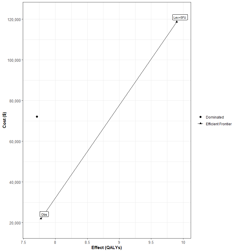
This work has been conducted under KD’s past affiliation and that GSK has no role in it↩︎