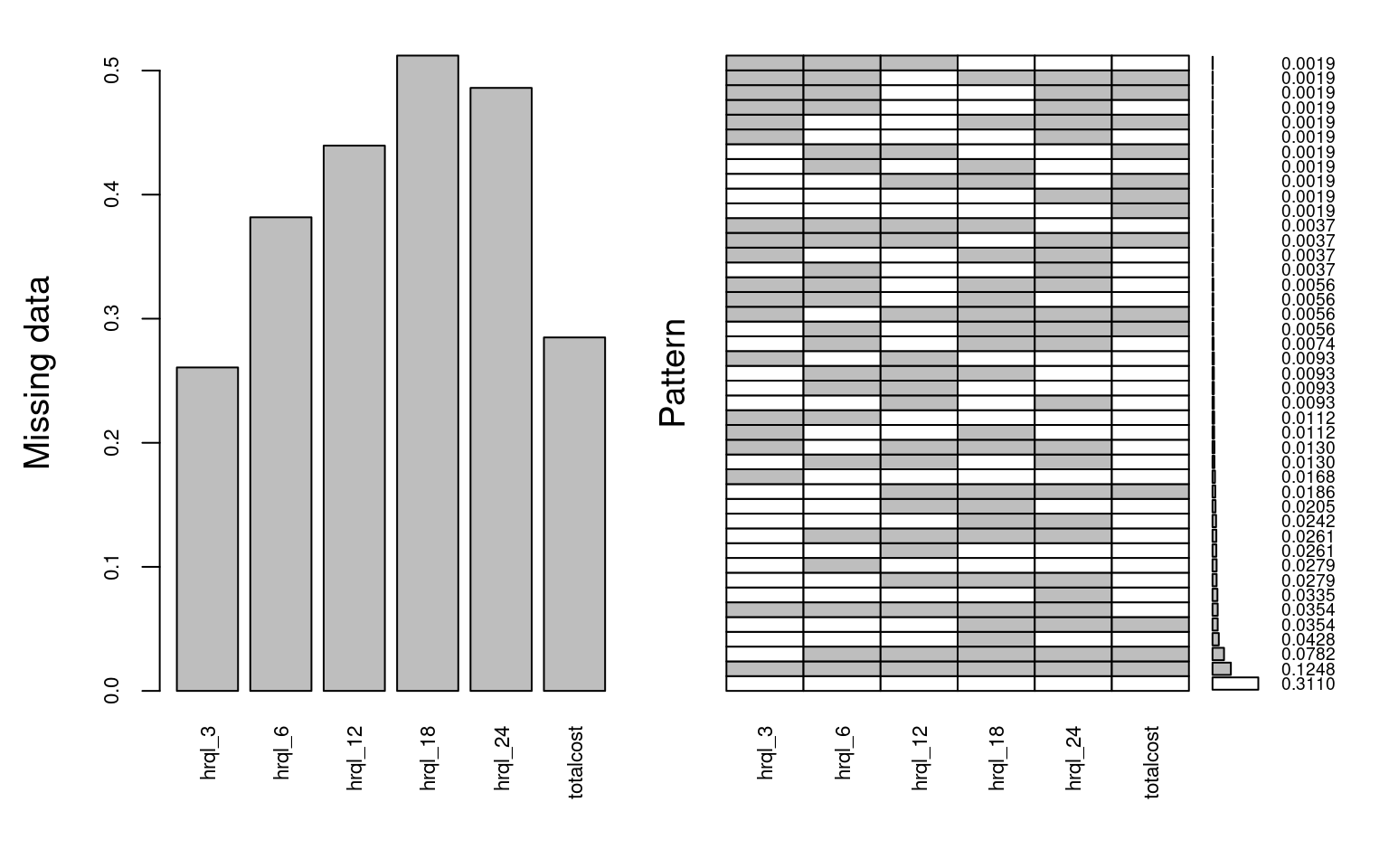
# missing data patterns
mice_plot <- VIM::aggr(
  data[,7:12], col=c('white','grey'), numbers=TRUE, sortVars=FALSE,
  cex.numbers=0.6, labels=names(data[,7:12]), cex.axis=.7, gap=3,
  ylab=c("Missing data","Pattern")
)
Andrea Gabrio
Maastricht University, Netherlands
Alexina Mason
London School of Hygiene and Tropical Medicine, UK
Baptiste Leurent
University College London, UK
Manuel Gomes
University College London, UK
Missing data are a common problem that complicates the statistical analysis of data collected in almost every discipline. This is also true for health economic evaluations based on individual-patient data, e.g. conducted alongside a randomised controlled trial (RCT), in which almost inevitably some individuals in the sample have their cost and/or effectiveness observations missing at one or more occasions of the follow-up. This issue is particularly pronounced in health economics where analyses rely on collecting rich, longitudinal information from participants, such as their use of healthcare services and their related health‐related quality of life. Study participants may, for example, drop-out of the study before its completion, miss a schedule visit, or leave blank some of the items of a questionnaire (Little et al., 2012).
Several reviews and guidelines have been published in recent years on the issue of missing data handling in the context of trial-based cost-effectiveness analysis (Diaz-Ordaz et al., 2014a; Faria et al., 2014; Gabrio et al., 2017; Leurent et al., 2018a; Noble et al., 2012). Most of these highlighted a general lack of compliance for standard practice with respect to missing data recommendations from the literature in several aspects, including poor reporting, assumptions justification and sensitivity analysis choices. When not properly handled, missing data may undermine the validity of economic evaluations and lead to incorrect evidence for healthcare decision making.
When some observations are missing, the collected data become incomplete in that some intended measurements could not be obtained. When the data from a study are incomplete, there are important implications for their analysis. First, the reduction of the available number of observations causes loss of information and a decrease in the precision of the estimates, which is directly related to the amount of missing data (Rubin, 2004). Second, missing data can introduce bias, resulting in misleading inferences about the parameters of interest. More specifically, the validity of any method is dependent on untestable assumptions about the reasons why missing values occur being true. As a result, caution is required in drawing conclusions from the analysis of incomplete data and the reasons behind any missingness must always be carefully considered.
Before conducting any analysis with incomplete data, it is important to understand a number of aspects of the missingness to guide the choice of appropriate methods to handle them. This can be achieved by answering three general questions: where (patterns of missing values); how much (amount of missingness); why (reasons for the missing data). The first two questions are typically straightforward to answer, given that the necessary information can be retrieved from the dataset itself. However, understanding the reasons for the missingness is a more challenging task.
We introduce some notation and terminology for missing data, with a focus on longitudinal study designs, which are often the source of cost-effectiveness data. Specifically, we assume that for each of \(N\) individuals, we intend to collect \(J\) repeated measures of the outcome variable and we denote with \(\boldsymbol Y=(Y_{1},Y_{2},\ldots,Y_{J})\) the outcome vector of a subject with a full set of responses. In general, \(Y_{ij}\) denotes the measurement collected for the \(i\)-th subject at the \(j\)-th time in the study, where \(i=1,\ldots,N\) and \(j=1,\ldots,J\). In addition, for each individual, associated with \(\boldsymbol Y\) there is a \(P\) matrix of covariates \(\boldsymbol X=(X_{1},X_{2},\ldots,X_{P})\), typically measured at baseline.
In the statistical literature the set of observations \(\boldsymbol Y\) that were intended to be collected and analysed is typically referred to as the complete data (i.e. data that would have been observed if no missingness occurred). However, in practice, for at least some individuals, some elements of \(\boldsymbol Y\) are not observed. For a given individual, we let \(\boldsymbol R=(R_{1},R_{2},\ldots,R_{J})\) be the vector of missing data indicators of the same length as \(\boldsymbol Y\) such that \(R_{j}=1\) if \(Y_{j}\) is observed at time \(j\) and \(R_{j}=0\) otherwise, for \(j=1,\ldots,J\).
Given \(\boldsymbol R\), the complete data \(\boldsymbol Y\) can be partitioned into the two components \(\boldsymbol Y^o\) and \(\boldsymbol Y^m\), respectively indicating the observed and missing set of outcome data. The joint set of the complete data and missingness indicators \((\boldsymbol Y,\boldsymbol R)\) is usually referred to as the full data whose density can be written as \[ f(\boldsymbol Y, \boldsymbol R \mid \boldsymbol X, \boldsymbol \theta, \boldsymbol \pi), \tag{6.1}\] where \(\boldsymbol X\) denotes the set of fully-observed covariates for \(\boldsymbol Y\), while \(\boldsymbol \theta\) and \(\boldsymbol \pi\) indicate the sets of parameters indexing the model for the outcome data and the missingness indicators, respectively. For example, in a simple regression framework, \(\boldsymbol \theta\) from Equation 6.1 can be decomposed into an intercept and slope coefficients \((\alpha, \beta)\) that relate the mean of \(\boldsymbol Y\) to \(\boldsymbol X\).
A first important distinction is whether missingness affects the outcomes (e.g. costs and effects) or the covariates. In the context of trial-based analyses, outcome data are typically collected at a set of time points, while covariates are often available only at baseline. Missing outcome data have historically been the most prominent and frequent type of missingness in economic evaluations, either in terms of costs (Briggs et al., 2003; Burton et al., 2007; Graves et al., 2002; Lambert et al., 2008; Oostenbrink et al., 2003), effects (Rombach et al., 2016; Simons et al., 2015), or both types of variables (Härkänen et al., 2013; Mason et al., 2017; O’Hagan and Stevens, 2001). In contrast, covariate data are often collected with more limited amounts of missing values, especially in the context of randomised controlled trials (Faria et al., 2014). Throughout this chapter, we will therefore focus on the description of issues and methods related to the analysis of missing individual-level outcome data, although missingness in the covariates will be touched upon lightly. Therefore, unless stated otherwise, the covariate data will be assumed to be fully-observed for all individuals in the analysis.
A second important aspect to consider before conducting the analysis is to check the amount and pattern of missing data, which are likely to provide some preliminary information about the magnitude of the potential impact of missing data uncertainty on the inferences. Depending on which outcome variable and at which occasions missingness occurred, different missing data patterns may arise. For example, when a missing observation at time \(j\) implies that all observations measured at subsequent occasions are also missing, then missingnes is refereed to as dropout. Dropout is a special case of monotone pattern of missingness, which can be formally defined as when there is a permutation of the measurement occasions such that a measurement earlier in the permuted sequence is observed for at least those subjects who are observed at later measurements. All other patterns of missingness are referred to as non-monotone (e.g. when intermittent missingness occurs). In general, dropout has been found to be quite frequent in most trial-based economic evaluations, particularly with respect to cost data (Oostenbrink and Al, 2005). However, the presence of differences in dropout rates between treatment groups or different types of non-monotone patterns within each group may have considerable implications and should be carefully considered when exploring the plausibility of missingness assumptions (Leurent et al., 2020).
When missingness is only due to dropout, i.e. no other missing data patterns occurs in the analysis sample, then the missing longitudinal outcome indicators \(\boldsymbol R\) can be replaced by scalar indicator \[D=1+\sum_{j=1}^JR_{j}, \tag{6.2}\] which denotes the occasion at which dropout occurs for each individual, and can also be thought as the length of the measurement sequence plus one. The representation of missingness given in Equation 6.2 is particularly useful for simplifying the task of modelling and formulate assumptions about the missingness process.
A third, and also the most important, aspect to take into consideration when analysing incomplete data, is to think about possible reasons for the missingness. Why subjects dropped out from the study? Are reasons likely to be different between missingness patterns, treatment groups and type of outcome variables? Do the subjects who dropped out have similar characteristics to individuals who remained in the study (also known as completers)? Any sort of information that helps answering these questions may be key in order to determine the plausibility of the missingness assumptions in the context considered and guide the choice of the methods. This is particularly important in the context of trial-based health economic analyses where outcome data are typically collected via self-reported questionnaires, such as CSRI (Beecham et al., 2001) for costs and EQ-5D (Balestroni and Bertolotti, 2012) for health-related quality of life, which are naturally prone to missingness. For example, individuals may decide to skip some items in a questionnaire because of bad instructions provided or too many questions asked, or they may be unwilling to answer all items because the topic of research is considered a threat to privacy.
Therefore, investigating possible reasons behind missing data becomes a crucial element in the analysis to quantify the uncertainty associated with the missed responses. This can be formally translated into questions about the process responsible of missingness, often referred to as the missing data mechanism (Rubin, 2004), and its implications and links to the data generating process. The missing data mechanism describes the probabilistic process which determines the chance that an observation is missing. Different “classes” or types of mechanisms can be defined according to different assumptions about how \(\boldsymbol R\) is related to \(\boldsymbol Y\) and \(\boldsymbol X\). Based on Rubin’s taxonomy (Rubin, 2004), three general classes of missingness mechanisms can be identified. Each of these classes is associated with different reasons for missingness and have therefore implications in terms of the appropriateness of different methods of analysis.
Missing Completely At Random (MCAR), where missingness is independent of both any observed or unobserved data. For example, a MCAR mechanism arises when a sample of patient questionnaires is lost and therefore any missing value is exclusively due to random chance. Two important conclusions can be drawn under MCAR: first, the completers can be thought as a random sample of the target population; second, any method that yields valid inferences in the absence of missingness will also yield valid (but inefficient) inferences using the completers alone.
Missing At Random (MAR), where missingness is independent of both any unobserved data after conditioning on the observed data. An example of a MAR mechanism is when an individual is removed from a study as soon as the value of a specific observed variable (e.g. age or BMI) falls outside a pre-specified range. Missingness is therefore under the control of the investigator and is related to some observed components. The MAR assumption has the following important implications: first, the completers are not a random sample from the target population and any analysis restricted to them will yield biased inferences; second, provided the parameters indexing the missingness process are “distinct” from those of the data process, the missing data mechanism is referred to as ignorable. This implies that the missing values can be validly “predicted” using the observed data and a correct model for the joint distribution of \(\boldsymbol Y\).
Missing Not At Random (MNAR), where missingness depends on some unobserved data even after conditioning on the observed data. A MNAR mechanism is often referred to as non-ignorable missingness because the missing data mechanism cannot be ignored but must be explicitly modelled in order to make inferences about the distribution of the complete data. We note that the term informative missingness is also sometimes used to describe MNAR mechanisms since the model assumed for \(\boldsymbol R\) is critical and can drive the results of the analysis.
Data are said to be MCAR when the probability that the observations are missing is unrelated to either any observed or missing values. More formally: \[\begin{equation*} \text{Pr}(\boldsymbol R \mid \boldsymbol Y^o, \boldsymbol Y^m, \boldsymbol X) = \text{Pr}(\boldsymbol R). \end{equation*}\] This amounts to assuming that there is no systematic difference between individuals with partially and fully observed data.
Data are said to be MAR when the probability that the observations are missing is related to some observed values but is unrelated to any missing values. Formally: \[\begin{equation*} \text{Pr}(\boldsymbol R_i \mid \boldsymbol Y^o_i, \boldsymbol Y^m_i, \boldsymbol X_i) = \text{Pr}(\boldsymbol R_i \mid \boldsymbol Y^o_i, \boldsymbol X_i). \end{equation*}\] Under MAR, any systematic difference between individuals with partially and fully observed data can be fully explained based on observed data.
Finally, data are said to be MNAR when the probability that the observations are missing is related to both some observed values and missing values \[\begin{equation*} \text{Pr}(\boldsymbol R \mid \boldsymbol Y, \boldsymbol X) = \text{Pr}(\boldsymbol R \mid \boldsymbol Y^o, \boldsymbol Y^m, \boldsymbol X). \end{equation*}\]
It is important to clarify that any assumptions made about the missingness process can never be verified from the data at hand, i.e. the observed data provide no information that can either support or reject a specific assumption about the mechanism over another. Because of this, identification is driven by unverifiable assumptions and conducting sensitivity analyses becomes a crucial task (Gabrio et al., 2020; Manca and Palmer, 2005; Mason et al., 2018). Indeed, the sensitivity of inferences to a set of plausible assumptions concerning the missingness process should always be carefully assessed (Gabrio et al., 2020; Leurent et al., 2018b).
There are many different statistical approaches to deal with missingness, each relying on different assumptions. We will broadly describe some of these techniques, with a focus on those that have been applied in economic evaluations. A more in-depth and complete presentation of the available methods can be found in the missing data literature (Molenberghs et al., 2014; Schafer and Graham, 2002).
Two broad classes of methods to handle missing data can be distinguished, namely ad-hoc methods and statistically principled methods, according to how the underlying missing data assumptions are formulated. On the one hand, ad-hoc methods derive inferences based on missing data assumptions that are implicitly formulated and that are difficult to evaluate. On the other hand, statistically principled methods are those based on a well-defined statistical model for the complete data, and explicit assumptions about the missing data mechanism. Within each of these two classes, methods can be further grouped based on the approach used to handle missingness.
Among ad-hoc methods, popular approaches include case deletion (CD) and single imputation (SI) methods. In CD methods, incompletely recorded units are simply discarded and the analyze is performed only on the units with complete data. When only data from the completers are used, the method takes the name of complete case analysis (CCA), and may be satisfactory with small amounts of missing data. However, in general, CCA can lead to serious biases and may cause large portions of the sample to be discarded. Despite their well-recognised limitations, CD methods historically represented the default missing data methods in economic evaluation mostly because of their ease of implementation (Gabrio et al., 2017; Leurent et al., 2018a). SI methods fill in each missing value once, and the resultant completed data are analyzed by standard methods. Commonly used procedures for single imputation include: hot-deck imputation, mean imputation, regression imputation, and last observation carried forward (Little and Rubin, 2019). These methods have also been used quite frequently to handle partially observed trial data, especially in the context of multi-item questionnaires to allow the computation of total scores (Rombach et al., 2016). However, these methods rely on quite restrictive assumptions (i.e. even stronger than MCAR sometimes), and always fail to account of the uncertainty underlying the imputation process.
Two main types of statistically principled methods can be distinguished, namely multiple imputation (MI) and fully Bayesian (FB) methods. Both approaches have been applied to health economic evaluations and can provide a well-defined statistical model and explicit missingness assumptions to generate stochastic information about the missing values and/or the missingness mechanism. Compared to ad-hoc methods, these approaches are computationally more complex but rely on less restrictive assumptions (Gomes et al., 2013; Mason et al., 2018). A detailed presentation of the assumptions, methodology and key features of MI and FB methods, with a focus on health economic applications, is provided in Section 6.3.
Although the choice of the missing data method is crucial, it is also of equal importance that the model for the full data distribution is specified so to take into account the statistical idiosyncrasies that affect both effect and cost data. Examples include: imbalances in baseline variables between treatment groups (Manca et al., 2005; Van Asselt et al., 2009); the correlation between the outcomes at both the patient level (Gabrio et al., 2021; O’Hagan and Stevens, 2001) and cluster level (Gomes et al., 2012; Ng et al., 2016); the high level of skewness characterising quality of life and, especially, cost data (Basu and Manca, 2012; Diaz-Ordaz et al., 2014b; Thompson and Nixon, 2005); the presence of spikes at one or both of the boundaries of the range for the underlying outcome distribution, e.g. null costs or perfect health states (Baio, 2014; Gabrio et al., 2019). In addition, when missingness arises, the choice of the analysis model is complicated by the fact that the fit of the models cannot be checked against the unobserved values and the robustness of the results to alternative specifications and missingness assumptions should be investigated in sensitivity analysis (Gabrio et al., 2019; Leurent et al., 2020).
Given the numerous statistical issues that characterise the health economic framework, we argue that, compared to ad-hoc methods, principled missing data methods provide a more flexible and robust approach to quantify the impact of missing data uncertainty on the final conclusions. They allow to specify and model the impact missing data may have on both outcomes, their dependence structure, and how these are translated in terms of changes in cost-effectiveness assessments is a major challenge. In the following sections we will provide a more in-depth examination of the advantages and limitations of two of these principled approaches, namely MI and FB, and how they can be implemented to handle missingness in economic evaluations.
The rest of the chapter is structured as follows. In Section 6.4, we present the case study used as motivating example and describe the main features of the data. Section 6.3 introduces the substantive model for the health economic analysis and briefly outlines how this can be used in the presence of missing data either using a multiple imputation or Bayesian approach. Section 6.8 applies MI and Bayesian methods to the motivating example and shows the R code used to implement each approach, especially for the purpose of conducting sensitivity analysis. Finally, Section 6.9 summarises our conclusions.
Our motivating example draws on the case-study described in the previous chapter — the Ten Top Tips (10TT) trial (see Chapter 5). Briefly, this study was a two-arm, individually randomised, controlled trial of a weight-loss intervention for obese adults attending general practices in the UK (Beeken et al., 2017). The intervention comprised self-help material delivered by a practice nurse, providing the patients with a set of ten simple weight-control behaviours, with strategies to make them habitual. The participants were randomised to receive either the 10TT intervention, or care as usual from their general practices. Health-related quality of life (HRQL; see Chapter 1) was measured by EQ-5D-3L questionnaires (Rabin and de Charro, 2001), completed at baseline and 3, 6, 12, 18 and 24 months. Costs were measured from the National Health Service (NHS) perspective over the 2-year study period and based on the intervention costs and the health resource use data collected from the practice records at the end of the trial. A within-trial cost-effectiveness analysis (CEA) was conducted and reported in details elsewhere (Patel et al., 2018).
In the CEA of the 10TT study, missing data was mostly driven by incomplete HRQL and cost data. All baseline covariates, including baseline EQ-5D-3L, were fully observed. The HRQL measure was somewhat incomplete across the different follow-up times. The 2-year QALYs (Chapter 1), calculated using the “area under the curve” approach based on the individual HRQL scores, was missing for individuals whose EQ-5D-3L was missing at any time point. Resource use data, derived from the GP records, were also incomplete for some participants. For simplicity, and unlike the previous chapter, we focus on the aggregated total cost at 2 years. This was mainly due to missing data patterns (and anticipated mechanisms) being fairly similar across the different cost components. In such settings, we do not expect major advantages of applying the missing data methods to the individual components (Mainzer et al., 2021; Rombach et al., 2018).
The trial recruited 537 participants, but only 148 (27.6%) fully completed the follow-up at two years. A substantial proportion of the missing data was due to patients dropping out of the study as some point during the follow up period (monotone missingness). Other individuals failed to complete interim follow up questionnaires at a specific time point (non-monotone missingness). The full breakdown of the extent of the missing data across the different variables is shown in Figure 6.1. There are many ways of describing the missing data in R, including using md.pattern() within the mice package, but here we suggest the function aggr from the VIM package as it nicely summarises both the proportion of missing data and the different patterns.
# missing data patterns
mice_plot <- VIM::aggr(
data[,7:12], col=c('white','grey'), numbers=TRUE, sortVars=FALSE,
cex.numbers=0.6, labels=names(data[,7:12]), cex.axis=.7, gap=3,
ylab=c("Missing data","Pattern")
)The left-hand side panel reports the proportion of individuals with incomplete data across the different variables. For example, total cost is missing for about 30% of the trial participants, while the % of incomplete EQ-5D-3L increases over time up to over 50%. The right-hand side panel shows the % of complete cases (27.6%), as well as the % of individuals within each combination of missing variables (patterns). For example, 11.6% had missing data for all the HRQL and cost variables, whereas about 5% of patients failed to complete any of the HRQL questionnaires but their costs were observed.
Table 6.1 reports patients’ characteristics according to their missingness status, by trial arm. In the control group, patients with missing data tended to be younger, more likely to be male and obese, and had relatively lower quality of life compared to the complete cases. These associations were relatively similar for patients in the treatment arm, except for sex where patients with missing data were more likely to be female compared to complete cases.
| Variable |
Control
|
Treatment
|
||||
|---|---|---|---|---|---|---|
| N | Mis N = 1721 |
Obs N = 1001 |
N | Mis N = 1981 |
Obs N = 671 |
|
| age | 272 | 55.61 (13.93) | 58.61 (11.24) | 265 | 54.96 (12.67) | 59.24 (11.02) |
| sex | 272 | 265 | ||||
| M | 53 (31%) | 35 (35%) | 66 (33%) | 17 (25%) | ||
| F | 119 (69%) | 65 (65%) | 132 (67%) | 50 (75%) | ||
| bmi | 272 | 265 | ||||
| < 35 | 85 (49%) | 57 (57%) | 88 (44%) | 32 (48%) | ||
| >= 35 | 87 (51%) | 43 (43%) | 110 (56%) | 35 (52%) | ||
| hrql_0 | 272 | 0.77 (0.22) | 0.78 (0.24) | 265 | 0.71 (0.28) | 0.73 (0.26) |
| 1 Mean (SD); n (%) | ||||||
The primary cost-effectiveness analysis assumed that, conditional on these patient characteristics and on the observed/available follow-up data, the probability of observing the data was unrelated to unobserved values (MAR assumption). It is recognised, however, that in weight loss trials participants who end up dropping out of the study tend to have relatively poorer health status. This means that the chance of observing cost-effectiveness endpoints, such as HRQL, may depend on unobserved values (partially observed health status), i.e. data are likely to be MNAR. It is therefore important to assess the extent to which cost-effectiveness results may differ according to different assumptions regarding the missing data, including plausible MNAR mechanisms. We will explore this in Section 6.5.3 and Section 6.8.4.
Multiple imputation (MI) (Rubin, 2004) involves replacing each missing observation with a set of plausible imputed values, drawn from the posterior predictive distribution of the missing data given the observed data. MI can be seen as an extension of ‘regression imputation’ (or single imputation), which fills in the missing observations with a single predicted value. Single imputation assumes that the imputed values are known rather than estimated, and hence, it underestimates the standard errors and distorts the correlation structure of the data. Unlike single imputation, MI draws multiple plausible values for each missing observation, recognising the uncertainty associated with both the missing data and estimated parameters in the imputation model. The more uncertain the imputation is (in terms of prediction of the unobserved value), the larger differences will be generated from one imputed dataset to another. MI relies on the correct specification of the imputation model.
Univariate imputation. Suppose we would like to impute the missing values in a single variable \(\boldsymbol Y\) conditional on a set of complete variables \(\boldsymbol X\). The MI procedure follows three steps:
Step 1 - Apply a regression model (see Section 4.6) \(f(\boldsymbol Y\mid \boldsymbol X)\) to the observed data to predict plausible values for the missing observations. This step involves: i) randomly drawing the regression parameters from their estimated sampling distribution, and ii) drawing values from their posterior predictive distribution to impute missing observations.
Step 2 - Use predicted values from Step 1 to fill in the missing values in \(\boldsymbol Y\). This process (steps 1 and 2) is repeated \(M\) times (\(M\) being the number of imputations) to create \(M\) imputed (complete) datasets.
Step 3 - Apply substantive model to each dataset independently to estimate the quantity of interest, for example, mean cost and QALY differences between treatment groups over the trial time horizon)
Step 4 - Combine the estimates obtained from the multiple datasets using Rubin’s rules to produce an overall mean estimate of the parameter of interest together with its standard error. Rubin’s rules ensure that the standard error reflects the variability within and across imputations.
To impute an incomplete continuous variable \(Y\) conditional on \(X\) we often use a linear regression model (assuming \(Y\) is Normally distributed):
Step 1 - Fit linear regression using complete cases to obtain \(\hat{\beta}\) and \(\hat{\sigma}\):
\[\begin{eqnarray*}\label{eq-step1-mi} (\boldsymbol Y | \boldsymbol X, \boldsymbol \beta) &\sim& N(\boldsymbol \beta \boldsymbol X, \boldsymbol \sigma^2) \end{eqnarray*}\]Draw \(\boldsymbol \beta^*\),and \(\boldsymbol \sigma^*\) from their estimated sampling distribution.
\[\begin{eqnarray*} \boldsymbol \sigma^{2*} &\sim& \hat{\boldsymbol \sigma}^2 (N_{obs} - k)/g \end{eqnarray*}\] where g is a random draw from standard Chi-2 distribution on \((N_{obs} - k)\) degrees of freedom.
\[\begin{eqnarray*} \boldsymbol \beta^* &\sim& N(\hat{\boldsymbol \beta}, \boldsymbol \sigma^{2*} (\boldsymbol X^T \boldsymbol X)^{-1}) \end{eqnarray*}\]Step 2 - Impute values for each missing observation in \(\boldsymbol Y\) as
\[\begin{eqnarray*} \boldsymbol Y &=& \boldsymbol \beta^* \boldsymbol X + \boldsymbol \epsilon^* \end{eqnarray*}\] where \(\epsilon^*\) is a random draw from \(N(0,\boldsymbol \sigma^{2*})\). We repeat Steps 1 and 2 \(M\) times to create \(M\) imputed datasets.
Step 3 - Apply the substantive model, \(f(\boldsymbol Y| \boldsymbol X)\), to each multiple imputed dataset to estimate the quantity of interest, say a regression coefficient \(\theta\).
Step 4 - Combine the estimates obtained across the \(m=1,\ldots,M\) imputed datasets to obtain \(\hat{\theta}\) and its variance \(V(\hat{\theta})\) using Rubin’s rules:
\[\begin{eqnarray*} \hat{\theta} &=& \sum_{m=1}^M \hat{\theta}_{m}\\ V(\hat{\theta}) &=& W + (1+1/M)B \end{eqnarray*}\]where the total variance is a linear combination of the is the within-imputation variance, \(W=(1/M) \sum_{m=1}^M W_m\), and is the between-imputation variance, \(B=(1/(M-1)) \sum_{m=1}^M (\hat{\theta}_{m}-\hat{\theta})^2\).
Imputing multiple variables. There are two main MI approaches to address multiple variables with missing data. The first is known as multivariate or joint imputation (Schafer, 1997). A joint multivariate model is fitted to the data, and values are drawn from a joint posterior distribution following the steps described above. Typically, this will be done using a multivariate normal model, with binary and categorical variables incorporated as latent Normal variables.
The second approach is known as MI by chained equations (MICE) or fully conditional specification (Raghunathan et al., 2001; Van Buuren, 2007). This approach involves fitting a univariate conditional model separately for each incomplete variable. All the missing values are first filled-in randomly, then each variable is imputed in turn, conditionally on all the other variables, and the “chained equations” cycle is repeated several times to converge and obtain one set of imputed data. As a different model is fitted for each variable, MICE can more flexibly accommodate its distributional nature; for example we can use linear regression for Normal continuous variables, semi-parametric approaches (e.g. predictive mean matching) to non-Normal continuous variables, or logistic regression for binary variables (White et al., 2011). In practice, joint and chained equations MI are likely to give asymptotically similar results, but the latter is more commonly used and we will focus on illustrating that approach in Section 6.6.
MI will be valid under MAR conditional on the variables included in the imputation model. Hence, it should include all the variables that are associated with missingness, for example socio-demographic characteristics of the patients. The imputation should also include all the variables in the analysis model, such as the outcomes (cost and effectiveness) and the adjustment covariates of the analysis model. This should of course include the treatment arm, although a recommended alternative is to impute separately the data by arm. As well as including all variables in the analysis model, the imputation model must also include covariates in an appropriate way with respect to the functional form. In other words, the imputation model should be at least as “rich” as the analysis model.
For example, if the analysis model includes non-linear terms or interactions, these should be reflected in the imputation as well. For summary variables, for example the total cost based on multiple items, including all the item variables is usually not necessary, except if the pattern of missingness differs between items. If two items have different pattern of missingness then it will be more efficient to include them separately in the model to avoid losing information and potentially less restrictive missing data assumptions.
The number of imputations necessary to obtain reliable imputed values will depend primarily on the amount of missing data. Ideally one would want the Monte Carlo error to be less than half the last decimal place reported. This should ensure the results remain stable if were to conduct a new set of imputations. In practice, this may requires too many imputations. Some have suggested to have a Monte Carlo error below 10% of its standard error (Von Hippel, 2020).
Other rules of thumb have been suggested, such as using the same number of imputations as the proportion of incomplete observations (White et al., 2011) or fraction of missing information, i.e. performing 20 imputations if proportion or fraction, respectively, is 20%. This may not be sufficient when imputing skewed variables with high variance, such as healthcare costs. In general, there is a trade-off to be considered between the computational effort required to perform the analysis and its robustness in terms of inference.
Standard MI is implemented under the MAR assumption, that is, conditional on the variables in the imputation model, missing data are expected to follow the same distribution as the observed data. However, this assumption may not always hold, and it is important to conduct sensitivity analysis to assess the robustness of the results to alternative missing data assumptions. There are two broad approaches to assess possible departures from MAR: selection models and pattern-mixture models.
Selection models specify the mechanism by which the data are observed, which is a function of the underlying data values. Selection models have the attractive feature that the missing data model can be directly incorporated into the analysis model, typically using a Bayesian framework (Daniels and Hogan, 2008). However, selection models make untestable assumptions about the conditional distribution of the unobserved data, and results can be very sensitive to departure from these assumptions (Gomes et al., 2020). This limitation is particularly relevant for CEA studies, as the cost and effectiveness endpoints tend to be difficult to parametrise (Mason et al., 2021).
The other approach is pattern-mixture models, which formulates the MNAR problem in terms of the different distributions between the missing and observed data. The overall distribution of a variable is seen as a mixture of a distribution when observed and a distribution when missing (“pattern-mixture,” Little, 1994). Pattern-mixture models have received increasing attention in CEA as they consider more easily interpretable parameters, such as the mean difference between missing and observed data Gabrio et al. (2020).
MI offers a flexible framework to conduct sensitivity analysis, particularly using the pattern-mixture framework. An MI approach commonly adopted in practice consists of simply modifying multiply-imputed datasets to reflect possible departures from the MAR assumption Leurent et al. (2018b). This can be done by using an “offset” parameter \(\delta\), representing the average difference between the missing and observed values, \(Y_{miss}=Y_{obs} + \delta)\). An alternative modification is to use \(\delta\) as a multiplicative “scale” parameter \(\phi\) so that \(Y_{miss}=Y_{obs}*\phi)\). For example, missing values could be assumed to be 10% lower than those observed, or \(\phi=0.9\).
The full MI procedure to conduct sensitivity analysis via pattern-mixture approach would involve the following steps:
Step 1 - Use MI to impute the missing values under a MAR assumption (as discussed in Section 6.5)
Step 2 - Modify the MAR-imputed data to reflect a range of plausible MNAR scenarios, for example by multiplying the imputed values by \(\phi\) , or by adding \(\delta\). This step is typically conducted over a range of plausible values for \(\phi\) or \(\delta\), assessing how alternative assumptions impact on the study’s conclusions. Approaches to inform the choice of values of theses parameters in practice is discussed elsewhere (Leurent et al., 2018b).
Step 3 - Analyse the resulting imputed datasets as usual, fitting the analysis model to each imputed dataset and combining the results using Rubin’s rules.
This approach is straightforward to implement in standard statistical software, and allows the impact of different MNAR mechanisms on the conclusion to be easily scrutinised and discussed, as we will illustrate in the next section.
In this section we illustrate the use of MI to address the missing data in the 10TT study, described in Section 6.4, using the mice package in R. We start by computing the QALY measure using the individual HRQL scores over time. For the purposes of the MI illustration, we then apply a simple linear transformation that shifts its distribution from left-skewed to right-skewed to facilitate the use of standard generalised linear models (e.g. assuming QALY follows a Gamma distribution — see Section 1.1 and Section 4.3.4 for more details, respectively) in the analysis.
# Calculate QALY based on the individual HRQL scores
# (using the 'area under the curve' approach)
data$qaly <- 0.125*data$hrql_0 + 0.25*data$hrql_3 + 0.375*data$hrql_6 +
                  0.5*data$hrql_12 + 0.5*data$hrql_18 + 0.25*data$hrql_24

# 1. We apply a simple linear transformation so that the QALY variable
#    shifts from left-skewed to right-skewed to facilitate the use of GLMs
data$qaly<- 3 - data$qalyWe start by setting up the different arguments required for the mice() function. Specifically, we start with a set-up run to generate initial values.
# Create a subset of the data that includes variables to be imputed and
# predictors sort data by treatment arm (1 - treatment, 0 - control)
data <- data[order(data$arm),]
data0 <- subset(
  data[data$arm=="control",],
  select=c(arm, sex, age, bmi, hrql_0, hrql_3, hrql_6, hrql_12,
           hrql_18, hrql_24, totalcost, qaly)
)
data1 <- subset(
  data[data$arm=="treatment",],
  select=c(arm, sex, age, bmi, hrql_0, hrql_3, hrql_6, hrql_12,
           hrql_18, hrql_24, totalcost, qaly)
)

ini  <- mice(data0, maxit=0)   #initial values
pred <- ini$pred    # 1 - used as predictor; 0 otherwise
meth <- ini$meth
The output above shows the default arguments used by the mice() function. The default imputation method for continuous variables is predictive mean matching (pmm), irrespective of its empirical distribution. The PredictorMatrix specifies which variables are used as predictors (1 if used as predictor, 0 otherwise) in which imputation models. Each row represents the imputation model for the variable in the rowname, although those variables with complete information (e.g. age and sex) will be ignored (not imputed). By default, all variables are used as predictors, unless the PredictorMatrix is customised.
In CEA, the endpoint measures are often derived from other variables used in the imputation model. For example, the variable qaly is a linear function of the HRQL measures. To ensure that the relationship (transformation) holds between the imputed values of the original variables and the transformed ones, we need to use passive imputation. Using the qaly as an example, we modify the imputation method to reflect the formula used to calculate the qaly. We also need to exclude qaly as a predictor from the imputation models for the HRQL variables to prevent any feedback (collinearity) in the imputation process.
# Modify imputation method for 'qaly' to perform 'Passive Imputation'
meth["qaly"] <- "~I(3 - (0.125*data$hrql_0 + 0.25*data$hrql_3 +
                    0.375*data$hrql_6 + 0.5*data$hrql_12 +
                    0.5*data$hrql_18 + 0.25*data$hrql_24))"

# exclude 'qaly' from predictors to prevent feedback
pred[c("hrql_0", "hrql_3", "hrql_6", "hrql_12", "hrql_18",
       "hrql_24", "totalcost"), "qaly"] <- 0

# exclude 'arm' from predictors as we are already imputing by arm
pred[c("hrql_0", "hrql_3", "hrql_6", "hrql_12", "hrql_18",
"hrql_24", "totalcost"), "arm"] <- 0 We then run the imputation with the adjusted PredictorMatrix. In this example, we considered 5 imputations and 10 iterations within each imputation, which allows us to keep Monte Carlo error below \(10\%\) of its standard error (Von Hippel, 2020).
# Perform multiple imputation using mice()
M <-5       # Change this to your desired number of imputations
imp0 <- mice(data0, m=M, meth=meth, seed=1710, pred=pred, maxit=10)
imp1 <- mice(data1, m=M, meth=meth, seed=1710, pred=pred, maxit=10)

imp <- rbind(imp0,imp1)   # combine imputations from the 2 arms
Next, we check the convergence of the MCMC chains by calling the function plot(), and decide whether we need more iterations. For example, we may check convergence using the following command
# Check convergence of MCMC chains
plot(imp, totalcost + qaly ~ .it | .ms, layout = c(2, 2))
Once we are happy with convergence, we can can perform a visual diagnostic of the plausibility of the imputed valued. Again, we can do this in many ways, for example using the densityplot() function in the mice package. Both totalcost and qaly are not Normally distributed, and using predictive mean matching helps MI to produce imputed values that reflect their empirical distributions.
# Assess plausibility of imputed values
densityplot(imp, ~totalcost + qaly, layout = c(1, 2))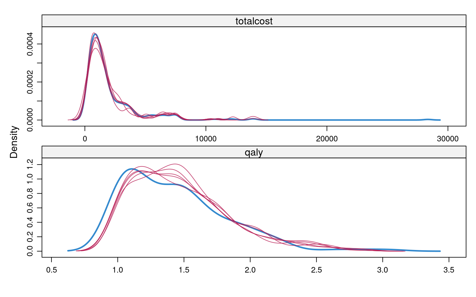
We have now checked the plausibility of the imputed values and are ready to analyse the imputed data. To fit the substantive model to the imputed datasets we do not need to stack them together, but instead use the option with() that loops over the imputed datasets in the object imp.
# Apply substantive model to data
mod.cost <- with(imp, glm(totalcost ~ arm, family = Gamma(link = "identity")))
mod.qaly <- with(
  imp, glm(qaly ~ arm + hrql_0, family = Gamma(link = "identity"))
)
We can apply Rubin’s rules and pool the results by using the pool() function.
# Apply Rubin's rules and estimate parameters of interest
# (incremental cost and QALY)
summary(pool(mod.cost), conf.int = TRUE)
term estimate std.error statistic df
1 (Intercept) 1808 132 13.71 386
2 armtreatment 440 222 1.98 149
p.value 2.5 % 97.5 % conf.low conf.high
1 0.0000000000000000000000000000000000379 1549.108 2068 1549.108 2068
2 0.0498506028551799276749001421649154508 0.291 879 0.291 879summary(pool(mod.qaly), conf.int = TRUE) term estimate std.error statistic df
1 (Intercept) 1.733 0.0609 28.45 183
2 armtreatment 0.120 0.0328 3.66 138
3 hrql_0 -0.444 0.0713 -6.23 184
p.value 2.5 %
1 0.00000000000000000000000000000000000000000000000000000000000000000000508 1.6131
2 0.00036058227925040364173631113331452979764435440301895141601562500000000 0.0552
3 0.00000000316574853127390655298414965258119169178030460898298770189285278 -0.5846
97.5 % conf.low conf.high
1 1.854 1.6131 1.854
2 0.185 0.0552 0.185
3 -0.303 -0.5846 -0.303Using \(5\) imputations, the incremental cost is \(\pounds 439.78\) (\(95\%\) CI \(\pounds 0.29\), \(\pounds 879.27\)) and incremental QALY is \(0.12\) (\(95\%\) CI is \(0.06\), \(0.18\))
In this section, we illustrate how to conduct MNAR sensitivity analyses using the pattern-mixture approach following MI, as described at the end of Section 6.5.3. In the 10TT study, we considered the MAR assumption to be plausible for the cost data (based on GP records) while patient-reported HRQL data was likely to be MNAR. We postulated that patients who dropped out of the study or failed to complete EQ-5D questionnaires were more likely to be in poorer health. We assumed that patients with missing HRQL had up to 0.1 lower EQ-5D-3L compared to that of individuals with fully observed HRQL data.
We considered different departures from the MAR assumption by subtracting \(\delta=(0.02, 0.04, 0.06, 0.08, 0.1)\) from the imputed values, where \(\delta=0\) corresponded to the MAR scenario. We first considered the same \(\delta\) across both randomised groups, and then allowed this parameter to differ by treatment arm. In the latter setting, we hypothesised that the magnitude of the utility decrement in the treatment group was half of that in the control arm, i.e. \(\delta=(0.01, 0.02, 0.03, 0.04, 0.05)\) for treatment arm.
The code below corresponds to scenarios in which the sensitivity parameter \(\delta\) is assumed constant across treatment arms. However, we can easily allow \(\delta\) to differ by treatment group, specifying a different post option for each treatment arm. Essentially, the post option provides a way of manipulating (post-processing) imputed values for a particular variable that are generated within each iteration.
post <- ini$post       # post option
d <- seq(0, 0.1,0.02)  # sensitivity parameter
est <- vector("list", length(d)) # list object to store results

# Re-run (post-process) MI for each MNAR scenario
for (i in 1:length(d)) {
  post["hrql_3"] <- paste("imp[[j]][,i] <- imp[[j]][,i] -", d[i])
  post["hrql_6"] <- paste("imp[[j]][,i] <- imp[[j]][,i] -", d[i])
  post["hrql_12"] <- paste("imp[[j]][,i] <- imp[[j]][,i] -", d[i])
  post["hrql_18"] <- paste("imp[[j]][,i] <- imp[[j]][,i] -", d[i])
  post["hrql_24"] <- paste("imp[[j]][,i] <- imp[[j]][,i] -", d[i])
  imp0 <- mice(data0, m=M, post=post, meth=meth, seed=1710, pred=pred, maxit=10)
  imp1 <- mice(data1, m=M, post=post, meth=meth, seed=1710, pred=pred, maxit=10)
  imp<-rbind(imp0,imp1)
  fit <- with(imp, glm(qaly ~  arm + hrql_0, family = Gamma(link = "identity")))
  est[[i]] <- summary(pool(fit), conf.int = TRUE)
}
Table 6.2 reports the full sensitivity analysis results. It suggests that the mean difference between treatment groups remains robust to plausible departures from MAR when \(\delta\) is assumed constant across the randomised groups. However, when we allowed \(\delta\) to differ between treatment arms, the incremental QALY increased substantially with the value of \(\delta\), becoming statistically significant when \(\delta=0.1\) for control arm and \(\delta=0.05\) for treatment arm.
| Same $\delta$ across trial arm | $\delta$ differs by treatment arm | |||||
|---|---|---|---|---|---|---|
| $\delta$ | Inc QALY | Lower CI | Upper CI | inc QALY | lower CI | upper CI |
| 0 (MAR) | -0.120 | -0.185 | -0.055 | -0.120 | -0.185 | -0.055 |
| 0.02 | -0.130 | -0.192 | -0.068 | -0.116 | -0.186 | -0.046 |
| 0.04 | -0.143 | -0.225 | -0.062 | -0.113 | -0.179 | -0.048 |
| 0.06 | -0.160 | -0.226 | -0.094 | -0.117 | -0.183 | -0.052 |
| 0.08 | -0.158 | -0.229 | -0.088 | -0.113 | -0.191 | -0.035 |
| 0.1 | -0.161 | -0.244 | -0.079 | -0.103 | -0.172 | -0.034 |
Bayesian inference (see Section 4.4.1) provides a principled way to account for uncertainty about the missingness while also ensuring its correct propagation through the specification of a fully-probabilistic model. We will make use of the case study introduced in Section 6.4 to demonstrate how the Bayesian approach can be implemented to handle missing data in economic evaluations and quantify their impact on cost-effectiveness conclusions. Many concepts of Bayesian inference are only briefly introduced for ease of presentation. For a more comprehensive introduction, we refer the interested readers to several monographs on Bayesian inference (Daniels and Hogan, 2008; Gelman et al., 2013; Jackman, 2009).
When applied to economic evaluation, the probabilistic framework characterising the Bayesian approach allows a flexible specification of the substantive model \(f(e,c \mid \boldsymbol \theta)\) via a series of simpler sub-models while preserving the multivariate relationships between the variables (Baio, 2012; Spiegelhalter et al., 2004). This is formally achieved through the factorisation of the joint distribution of effects and costs into the product of a marginal distribution for one variable and a conditional distribution for the other variable. For example, a possible factorisation of the substantive model is: \[f(e_{i},c_{i}\mid \boldsymbol \theta) = f(c_{i}\mid \boldsymbol \theta_c)f(e_{i}\mid c_{i}, \boldsymbol \theta_e), \tag{6.3}\] where \(f(c_{i}\mid \boldsymbol \theta_c)\) and \(f(e_{i}\mid c_{i} ,\boldsymbol \theta_e)\) denote the marginal distribution of the costs and the conditional distribution of the effects given the costs, respectively. The key advantage of Equation 6.3 is that models for \(e\) and \(c\), indexed by distinct parameter sets \(\boldsymbol \theta_e\) and \(\boldsymbol \theta_c\), can be separately specified in a flexible way. Distributional and modelling choices can then be tailored to the specific sub-model considered to take into account the features of each type of outcome data while preserving the multivariate relationship between the outcomes. In Section 6.8, we will explore and use this specification of the substantive model for the analysis of the economic data in our motivating example.
In many cases, economic evaluations are conducted without clear information about the likely values of the parameters of interest before observing the data. Within a Bayesian framework, this is translated into the specification of a weakly-informative or vague prior, such that the resulting posterior will be almost entirely informed by the likelihood function (see Figure 4.13 and Section 4.4.2). However, in some cases, it may be possible to incorporate into the model information about the parameters which comes from other sources. This corresponds to the specification of an informative priors which, together with the likelihood, drives posterior inferences. Informative priors may be derived from historic data or elicited from experts (Mason et al., 2017; O’Hagan, 2019; O’Hagan et al., 2006).
The Bayesian approach treats missing data as additional unknown quantities for which a posterior distribution can be estimated, i.e. there is no fundamental distinction between missing data and unknown parameters. Using again the missing data notation from Section 6.2: the data \((\boldsymbol Y^o,\boldsymbol X, \boldsymbol R)\) comprise the observed outcome, covariates and missingness indicators; the set of unobserved quantities \((\boldsymbol Y^m,\boldsymbol \theta)\) consist of the missing outcomes and model parameters.
For model-based inference with missing data, there is always an underlying joint model for the missingness and the outcomes \(f(\boldsymbol Y, \boldsymbol R \mid \boldsymbol X, \boldsymbol \theta,\boldsymbol \pi)\), where \(\boldsymbol \theta\) and \(\boldsymbol \pi\) denote the distinct sets of parameters indexing the analysis and missing data model, respectively. A convenient way to express the full data joint distribution is through the selection model factorisation as the product of the analysis model \(f(\boldsymbol Y \mid \boldsymbol X, \boldsymbol \theta)\) and the missing data mechanism \(f(\boldsymbol R \mid \boldsymbol Y, \boldsymbol X, \boldsymbol \pi)\). Ignorable missingness in Bayesian inference holds under the following three conditions: 1) the missing data mechanism is MAR; 2) the sets of parameters \(\boldsymbol \theta\) and \(\boldsymbol \pi\) are distinct; 3) The priors on the full data model parameters can be factored as \(f(\boldsymbol \theta, \boldsymbol \pi)=f(\boldsymbol \theta)f(\boldsymbol \pi)\) (a priori independence).
Under Bayesian ignorability, the posterior distribution of \(\boldsymbol \theta\) can be factored as \[\begin{equation*} f(\boldsymbol \theta \mid \boldsymbol Y^o,\boldsymbol R, \boldsymbol X) = f(\boldsymbol \theta \mid \boldsymbol Y^o,\boldsymbol X) f(\boldsymbol \pi \mid \boldsymbol R, \boldsymbol X), \end{equation*}\] so that inference on the model parameters \(\boldsymbol \theta\) only requires specification of the outcome model \(f(\boldsymbol Y \mid \boldsymbol X, \boldsymbol \theta)\) and the prior \(f(\boldsymbol \theta)\), since the distribution of the missing data \(f(\boldsymbol Y^m \mid \boldsymbol Y^o, \boldsymbol R)\) is identified under ignorability (Molenberghs et al., 2014).
From a computational perspective, to calculate posterior summaries (e.g. means or credible intervals), numeric integration methods are typically required. Among these, Markov Chain Monte Carlo (MCMC) methods are often used (Brooks et al., 2011). Very broadly, these methods aim at sequentially sampling from generic probability distributions, which are based on the construction of a Markov chain that converges to the target posterior (see also Section 5.4.4 for another application of Bayesian analysis). For a detailed presentation of different types of MCMC methods we refer the reader to the relevant literature (Brooks et al., 2011). Software specifically designed for the analysis of Bayesian analysis using MCMC techniques have been developed. This includes those based on the model description language known as BUGS (Bayesian inference Using Gibbs Sampling, Lunn et al., 2013), among which JAGS (Just Another Gibbs Sampler, Plummer, 2013) is our reference software choice that we use to fit all Bayesian models in this chapter.
RIn this section we show how to build a Bayesian model to handle missingness and derive the cost-effectiveness results using R and JAGS. Using the economic data from the case study described in Section 6.4, we start by describing stand-alone sub-models for the costs and the utilities, and then demonstrate how these can be combined into a joint model, assuming that the unobserved outcomes are MAR. Finally, we extend this model to allow some of the missing outcomes to be MNAR. Before proceeding, we load all the following R packages: denstrip, foreign, rjags, runjags, bayesplot, bayesplot, BCEA, ggpubr, ggridges and HDInterval.
We then load the dataset from a csv file into the object tenTT, for example, something like the following command.
tenTT <- read.csv(file="data/10TT_synth_280921_mg.csv", sep=",")Next we pre-process the variables to facilitate model fitting. Specifically, we recode the treatment group indicator to \(1\) (control) and \(2\) (intervention), standardise all baseline covariates (age, BMI and sex) and express cost data in thousands pounds. Finally, we create a list tenTT.data which incorporates all the variables needed to fit our first model.
arm <- tenTT$arm+1
age <- (tenTT$age - mean(tenTT$age))/sd(tenTT$age)
bmi <- tenTT$bmicat-1
bmi.c <- (bmi - mean(bmi))/sd(bmi)
sex <- tenTT$sex-1
sex.c <- (sex - mean(sex))/sd(sex)
Xs <- cbind(age,bmi.c,sex.c)
costs <- tenTT$totalcost
tenTT.data <- list(
  Np=length(arm), Nx=dim(Xs)[2], cost=costs/1000, X=Xs, tr=arm
)First, we consider a MAR model for handling missingness in total costs conditional on the observed covariates. We therefore specify a model \(f(c_{ik} \mid \boldsymbol X_{ik}, \boldsymbol \theta_c)\), where \(\boldsymbol X_{ik}\) and \(\boldsymbol \theta_c\) denote the set of baseline covariates included (i.e. age, sex and BMI) for individual \(i\) in treatment arm \(k\) and the parameters indexing the cost model respectively.
Since only total costs computed over the trial period are available, we specify a cross-sectional cost model that includes all available covariates to control for possible confounders and improve parameter estimation. We assume that the cost outcomes have a Gamma distribution with treatment-specific means and a common standard deviation. Since Gamma distributions are canonically defined in terms of shape and rate parameters, we re-express these parameters as functions of the mean to which we assign vague prior distributions.
For each individual \(i\) and treatment group \(k\), the model assumed for total cost variables \(c_{ik}\) is specified as follows: \[\begin{eqnarray*} c_{ik} &\sim& \text{Gamma}(a_{k}, b_{k}) \\ a_{k} &=& b_{k} \mu^c_{k} \\ \log(\mu^c_{t}) &=& \boldsymbol X_{k}\boldsymbol \zeta_{k}\\ b_{k} &=& \frac{a_{k}}{\mu^c_{k}}, \end{eqnarray*}\] where \(a_{k}\) and \(b_{k}\) are the shape and rate canonical parameters of the Gamma distribution, \(\mu^c_{k}\) is the cost mean, while \(\boldsymbol \zeta_{k}\) is the vector of regression parameters associated with the covariate matrix \(\boldsymbol X_{k}\), which includes an intercept, age, BMI and sex. Vague priors are specified on all model parameters. These include: independent Normal distributions centred at \(0\) and variance \(100\) for the regression parameters (defined on log scale) and weakly informative Gamma distributions on the shape parameters.
We can directly type the JAGS code of the model in R or save it in a separate .txt file in the current working directory. For example, we store the model code as a R string object named cost.gamma.mod.
## gamma analysis model for total costs
cost.gamma.mod <- "
# cost = total costs in £1000s
# treatment received is indexed by tr (1 = control and 2 = intervention)

model{
    for (i in 1:Np) { # loop through individuals with cost data
        cost[i] ~ dgamma(shape.c[tr[i]],rate.c[i])
        log(mu.c[i]) <- zeta0[tr[i]] + inprod(zeta[1:Nx,tr[i]],X[i,])
        rate.c[i] <- shape.c[tr[i]]/mu.c[i]
        # predicting cost assuming all participants receive treatment 1
        pred.c1[i] <- exp(zeta0[1] + inprod(zeta[1:Nx,1],X[i,1:Nx]))
        # predicting cost assuming all participants receive treatment 2
        pred.c2[i] <- exp(zeta0[2] + inprod(zeta[1:Nx,2],X[i,1:Nx]))
        Ctot.diff[i] <- pred.c2[i] - pred.c1[i]

    #get dataset predictions to compare
    cost.rep[i] ~ dgamma(shape.c[tr[i]],rate.c[i])
    }

    for (k in 1:2) { # 2 treatment arms
        # prior distributions
        zeta0[k] ~ dnorm(0,0.01)
        for (i in 1:Nx) {zeta[i,k] ~ dnorm(0,0.01)}
        shape.c[k] ~ dgamma(0.001,0.001)
    }

    # calculating cost increment using recycled predictions
    AveC[1] <- mean(pred.c1[])*1000
    AveC[2] <- mean(pred.c2[])*1000
    Cinc <- mean(Ctot.diff[])*1000
    p.Cinc <- 1-step(Cinc) # probability favours new treatment
}
"
We use the method of recycled predictions to predict the incremental cost (Basu and Manca, 2012; Mason et al., 2021). This method uses baseline covariates to predict the costs for all patients assuming they are randomised to receive usual care (pred.c1) and the ten top tips intervention (pred.c2), and the difference between the two outcomes predicted for each individual is then calculated (Ctot.diff). The mean total costs in each arm is then calculated as the average of the corresponding predictions (Avec), while the incremental effect is computed as the mean of these differences (Cinc). Finally, we calculate the proportions of simulations for which the incremental effect is less than zero (p.Cinc), indicating the probability of having a cheaper new treatment.
Next, we set initial values for the model parameters in each chain of the MCMC algorithm within the lists inits1 and inits2 (we run two chains) and type the names of the parameters we want to monitor inside the object pars. In the summary.pars object we only retain those parameters for which we want to print posterior summaries.
inits1 <- list(".RNG.name" = "base::Wichmann-Hill",".RNG.seed" = 12345)
inits2 <- list(".RNG.name" = "base::Wichmann-Hill",".RNG.seed" = 98765)
cost.inits1 <- c(list(zeta0=rep(0.5,2),zeta=matrix(rep(c(0.1,0.1,0.1),2),3,2),
               shape.c=c(1,1)),inits1)
cost.inits2 <- c(list(zeta0=rep(1,2),zeta=matrix(rep(c(-0.1,-0.1,-0.1),2),3,2),
               shape.c=c(3,3)),inits2)
cost.pars <- c("zeta0","zeta","shape.c","AveC","Cinc","p.Cinc","cost.rep")
cost.summary.pars <- c("AveC","Cinc","p.Cinc")
We then run the model using the run.jags function in the R package runjags and save the results in the object g1.out. We also need to provide additional information in relation to the MCMC algorithm, namely the number of chains, number of samples (to store), adaptive (to start) and burnin (to discard) iterations, and the thinning interval.
# run model
set.seed(123)
g1.out <- run.jags(
  model=cost.gamma.mod, monitor=cost.pars, data=tenTT.data, n.chains=2,
  inits=list(cost.inits1,cost.inits2), burnin = 1000, sample = 5000,
  adapt = 1000, thin=1, modules=c('glm','dic')
)
We use the summary command to summarise the posterior distributions for the monitored parameters in terms of means, medians, standard deviations and credible intervals.
# create summaries
g1.summary <- summary(g1.out,vars=cost.summary.pars)[,1:5]
Lower95 Median Upper95 Mean SD
AveC[1] 1611.950 1794.930 1993.430 1799.4730 99.25562163
AveC[2] 2009.380 2330.160 2683.560 2339.0332 173.99580951
Cinc 170.882 532.911 956.848 539.5602 202.02908257
p.Cinc 0.000 0.000 0.000 0.0026 0.05092641After running the model we check the convergence of the MCMC algorithm and the adequacy of the posterior sample used for inference. The convergence and effective sample size checks can be carried out using standard graphics and diagnostics, and so details are omitted here. Our checks were satisfactory. Residual plots provide one option for assessing the fit of the model with respect to the observed data. An alternative is to evaluate the model’s predictive accuracy: a typical approach uses posterior predictive checks (Gelman et al., 2013), in which simulated values are drawn from the posterior predictive distribution and compared to the observed data, either graphically or using discrepancy measures. Within R, the package bayesplot provides a set of functions to obtain many types of posterior checks aimed at comparing the observed and predicted data using different types of measures and plots, e.g. posterior densities. Examples of different types of posterior predictive checks that can be used to assess the model are provided in the R script in the electronic supplement.
We specify a longitudinal model \(f(q_{itk} \mid \boldsymbol X_{ik}, \boldsymbol \theta_e)\) for the effect variables (i.e. the health-related quality of life measurements \(q_{itk}\)) and use random effects to capture the temporal dependence across the five follow-up points. The model is specified under MAR conditional on the observed baseline covariates (i.e. age, sex and BMI). Since the quality of life measurements have a skewed distribution with a spike at 1 (i.e. perfect health), we specify a Gamma distribution with a hurdle component to handle the spike.
For each individual \(i\), follow-up point \(t\) and treatment group \(t\), the model assumed for the utility decrements \(u_{itk}\) is specified based on a hurdle or two-mixture components. Individuals are assigned to the first component when associated with zero utility decrements (structural component) and to the second component when associated with positive utility decrements (non-structural component). To ease notation, from now on we drop the treatment index \(k=1,2\), and formally present the model as: \[\begin{eqnarray*}
f(u_{it} \mid d_{it}=1) &=& f(u_{it} \mid \boldsymbol \theta^{0}_e) \\
f(u_{it} \mid d_{it}=0) &=& f(u_{it} \mid \boldsymbol \theta^{>0}_e),
\end{eqnarray*}\] where \(d_{it}\) is the zero decrement indicator for person \(i\) at time \(t\), while \(\boldsymbol \theta^{0}_e\) and \(\boldsymbol \theta^{>0}_e\) are the distinct parameter vectors indexing the structural and non-structural components of the utility mixture, respectively. The first component (\(d_{it}=1\)) is assigned a degenerate point mass distribution at \(0\), while the second component (\(d_{it}=1\)) is assigned a Gamma distribution with baseline utilities and other covariates included as predictors at the mean level. Within JAGS, we can succinctly re-write the model as: \[\begin{eqnarray*}
u_{it} &\sim& \text{Gamma}(a^{d}_{t}, b^d_{t}) \\
a^d_{t} &=& b^d_{t} \mu^d \\
\log(\mu^d_{t}) &=& \boldsymbol X\boldsymbol \beta^{d}_{t} + \omega \\
b^d_{t} &=& \frac{a^d_{t}}{\mu^d_{t}},
\end{eqnarray*}\] where \(a^{d}_{t}\), \(b^{d}_{t}\) are the shape and rate parameters, \(\mu^d_{t}\) is the conditional utility mean decrement, while \(\boldsymbol \beta^d_{t}\) is the vector of regression parameters associated with \(\boldsymbol X\). The superscript \(d\) denotes which component of the mixture each parameter is indexing, i.e. either the structural (\(d=1\)) or non-structural (\(d=0\)) part. The random term \(\omega\) is a normally distributed individual effect which is used to capture the temporal autocorrelation within the non-structural component of the model. The probability of having a zero decrement at each follow-up point is estimated as: \[\begin{eqnarray*}
d_{it} &\sim& \text{Bernoulli}(\pi_{t}) \\
\text{logit}(\pi_{t}) &=& \boldsymbol X\boldsymbol \gamma_{t}
\end{eqnarray*}\] where \(\pi_{t}\) is the probability of having a zero decrement and \(\boldsymbol \gamma_{t}\) is the vector of logistic regression coefficients associated with \(\boldsymbol X\). The overall mean utility decrement at each follow-up across both components is retrieved by computing the weighted means between the means from the two components of the mixture with weights given by \(\pi_{t}\) and \((1-\pi_{t})\). Next, the overall mean QALYs is obtained by applying the AUC formula to the marginal mean utility scores (i.e. 1 - mean decrement) estimated at each follow-up. Vague priors are specified on all model parameters indexing the non-structural component and the logistic regression.
Before implementing the longitudinal utility model in R and JAGS, some pre-processing of the data is required. First, we standardise the baseline utilities and include them as covariates in the model to control for possible baseline imbalances between treatment groups. Second, we create an outcome matrix qolmat containing the utility measurements collected at each follow-up point in the study and compute its complement qoldrec denoting the corresponding observed utility decrements. Converting the outcome variables in terms of utility decrements has the advantage that non-Normal distributions can be fitted quite easily to the transformed data (e.g. Gamma), which improves the fit of the model to the observed data. Third, we create the matrix of indicators hmat associated to whether a perfect score (i.e. null decrement) is observed for each individual at each follow-up point. These are used to assign individuals to the hurdle components of the model and separate the “structural” (i.e. zero decrement) from the “non-structural” component in the data.
# standardise baseline qol
bq <- tenTT$hrql_0
bq.c <- (bq - mean(bq))/sd(bq)

# create a matrix of EQ-5D measurements: 3, 6, 12, 18 and 24 months
qolmat <- cbind(tenTT$hrql_3,tenTT$hrql_6,tenTT$hrql_12,
                tenTT$hrql_18,tenTT$hrql_24)
qoldec <- 1-qolmat # calculate qol decrements
nts <- dim(qoldec)[2] # time-points
nps <- dim(qoldec)[1] # patients

hmat <- ifelse(qoldec==0,1,0) # hurdle indicator

epsilon <- 0.0001 # use to ensure q is positive for Gamma models
tenTT.data <- list(Np=nps, Nt=nts,  Nx=dim(Xs)[2], h=hmat,
                   q=qoldec+epsilon, bq=bq.c, X=Xs, tr=arm)
Next, we write the JAGS code for the longitudinal utility model within R and save it in the current working directory as a .txt file.
To ease presentation, here we briefly describe the structure of the model as defined within JAGS and provide the full model code in the R script in the electronic supplement. Similarly to the cost model, for the health-related quality of life (decrements) model we compute recycled predictions by treatment arm and, in this case, also by time point. We then apply the AUC formula to obtain recycled predictions in terms of QALYs by treatment arm and compute the difference between the two. Next, we proceed to obtain estimates of the mean QALYs by treatment arm and of the incremental effect by taking the average across the predictions (AveQ) and the differences (Qinc), and compute the probability for the new intervention to be more effective than the control (p.Qinc).
After generating the initial values for all model parameters in the list objects qol.inits1 and qol.inits1 (two chains), we select the parameters to monitor in the objects qol.pars and qol.summary.pars. We then run the model using the run.jags function and save the output in the object q1.out.
#run model
set.seed(123)
q1.out <- run.jags(model=qol.hurdle.mod, monitor=qol.pars, data=tenTT.data,
                   inits=list(qol.inits1,qol.inits2),
                   n.chains=2, burnin = 5000, sample = 1000, adapt = 1000,
                   thin=1, modules=c('glm','dic'))
Once the model has run, we summarise the posterior results for the selected parameters using the summary function
# show results
q1.summary <- summary(q1.out,vars=qol.summary.pars)[,1:5]
Lower95 Median Upper95 Mean SD
AveQ[1] 1.4192400 1.45002500 1.4816900 1.44971146 0.01625208
AveQ[2] 1.3811000 1.41986500 1.4598900 1.41929649 0.01981235
Qinc -0.0840691 -0.02946205 0.0174119 -0.03041498 0.02589509
p.Qinc 0.0000000 0.00000000 1.0000000 0.11550000 0.31970433We carried out similar checks as for the cost model, which suggested a generally good performance of the model. The interested reader can find details of some residual checks in the R code in the electronic supplement.
To conclude, we fit a joint model which combines the sub-models for the total cost and utility data, shown in Section 6.8.2 and Section 6.8.1 respectively. The model specified handles the different complexities of the data (e.g. skewness and structural values) while also accounting for the dependence between utilities and costs. Specifically, we factor the joint distribution of the two types of outcomes, ignoring treatment index to ease notation, as follows:
\[f(u_{it},c_{i} \mid \boldsymbol X_{i}, \boldsymbol \theta) = f(u_{it} \mid \boldsymbol X_{i}, \boldsymbol \theta_e) f(c_{i}\mid u_{it},\boldsymbol X_{i}, \boldsymbol \theta_c), \tag{6.4}\] that is the joint model is expressed in terms of a marginal distribution of the utilities at each follow up \(f(u_{it} \mid \boldsymbol X_{i}, \boldsymbol \theta_e)\) and a conditional distribution for the total costs given the utilities \(f(c_{i}\mid u_{it},\boldsymbol X_{i}, \boldsymbol \theta_c)\). Both models in Equation 6.4 are specified as before, with the only exception that the utilities are now included in the cost model to account for the dependence between the two types of outcomes. Thus, within the model, the conditional cost mean is now expressed as: \[\begin{equation*} \log(\mu^c) = \boldsymbol X\boldsymbol \zeta + \eta(e_{i}-\mu^e)\\ \end{equation*}\] where \(\eta\) is the regression parameter capturing the dependence between cost and the centred QALYs \((e_{i}-\mu^e)\), which are derived from the marginal utility hurdle specification as shown in Section 6.8.2.
After pre-processing the data, we proceed to write down the JAGS code of the model within R and save it in the object mar.mod1. The full model code can be found in the R script in the electronic supplement: here we only show changes made to the utilities and costs sub-models and additions to calculate incremental net benefits.
## joint model for costs and utilities
mar.mod1 <- "
model{
    # code for QoL marginal sub-model ---
    # full code available in the electronic supplement

    # Cost conditional sub-model
    for (i in 1:Np) { # loop through individuals with cost data
      # new code to calculate QALYS
        # switch from QoL decrements to QoL to calculate QALYs
        Qtot[i] <- 0.125*bq[i] + 0.25*(1-q[i,1]) + 0.375*(1-q[i,2]) +
        0.5*sum((1-q[i,3:4])) + 0.25*(1-q[i,5])
        Qmu[i] <- 0.125*bq[i] + 0.25*(1-pred.q[i,1]) + 0.375*(1-pred.q[i,2]) +
        0.5*sum((1-pred.q[i,3:4])) + 0.25*(1-pred.q[i,5])

        # new term added to link to QoL sub-model
        cost[i] ~ dgamma(shape.c[tr[i]],rate.c[i])
        log(mu.c[i]) <- zeta0[tr[i]] + inprod(zeta[1:Nx,tr[i]],X[i,]) +
        xi[tr[i]]*(Qtot[i]-Qmu[i])
        # remaining lines as before
    }

    for (k in 1:2) { # 2 treatment arms
        xi[k] ~ dnorm(0,0.01)
        # other priors specified as before
    }

    # code for converting to QALY diff over 2 year period ---
    # code for calculating QALY increment using recycled predictions ---
    # code for calculating cost increment using recycled predictions ---
}
"
The model combines the specifications shown for the total cost and health-related quality of life models into a single modelling framework. Key quantities that are stored into the R workspace include: the mean total costs and QALYs per treatment arm (AveC and AveQ), the incremental effects between arms (Cinc and Qinc) and the probabilities of having a cheaper and more effective new treatment compared to the control (p.Cinc and p.Qinc).
We then specify the initial values for the model parameters, and select those to monitor.
joint.inits1 <- c(cost.inits1,qol.inits1)
joint.inits1$xi <- c(-1,-1)
joint.inits2 <- c(cost.inits2,qol.inits2)
joint.inits2$xi <- c(-1,-1)
joint.pars <- c(cost.pars,qol.pars,"xi")
joint.summary.pars <- c(cost.summary.pars,qol.summary.pars)
Next, we run the model in R via the function run.jags and save it in the object j1.out.
#run model
set.seed(123)
j1.out <- run.jags(
  model=mar.mod1, monitor=joint.pars, data=tenTT.data, n.chains=2,
  inits=list(joint.inits1,joint.inits2),burnin = 5000, sample = 1000,
  adapt = 1000,thin=1,modules=c('glm','dic')
)
After running the model, we summarise the posterior results for key model parameters.
# show results
j1.summary <- summary(j1.out,vars=joint.summary.pars)[,1:5]
Lower95 Median Upper95 Mean SD
AveC[1] 1477.0362567 1650.67632122 1857.870396925 1653.13248116 98.99342146
AveC[2] 1803.8373914 2130.97191624 2486.137351162 2138.61329480 178.48713912
Cinc 95.0783863 476.92610180 880.501439380 485.48081364 204.74463998
p.Cinc 0.0000000 0.00000000 0.000000000 0.00400000 0.06313472
AveQ[1] 1.3860628 1.41766352 1.449020329 1.41721034 0.01644282
AveQ[2] 1.3384286 1.37922087 1.415793736 1.37855195 0.02005981
Qinc -0.0926594 -0.03945947 0.009991052 -0.03865839 0.02636130
p.Qinc 0.0000000 0.00000000 1.000000000 0.07050000 0.25605181Posterior results indicate a mean QALYs difference (Qinc) of \(-0.039\) with \(95\%\) credible interval ranging between \((-0.093, 0.01\), and a mean total costs difference (Cinc) of \(\pounds 485\) with \(95\%\) credible interval ranging between \((\pounds 95,\pounds 881)\). According to these results, the average probabilities that the new intervention is more effective (p.Qinc) and less expensive (p.Cinc) compared to the control are \(0.07\) and \(0.004\), respectively.
Exploring the sensitivity of the results with respect to different missingness assumptions is a crucial task in any analysis with partially-observed data since, by definition, missingness assumptions can never be checked from the data at hand. The specific missingness assumptions to explore should be defined according to the context of the analysis and outcome variables. For the 10TT trial, it seems likely that the probability of a patient providing their utility at a particular time point is related to their health status at that time, which would imply a MNAR mechanism. By contrast, it may be reasonable to assume that missingness in costs is due to administrative reasons and can therefore be assumed to be MAR. Therefore, in the following, we will extend the joint model described in Section 6.8.3 to assess the robustness of the results to some MNAR departures for the utility data. Alternative approaches can be used to explore MNAR departures and, in contrast to the pattern-mixture model shown in the context of multiple imputation in Section 6.5.3, here we show how selection models can be implemented within a Bayesian framework (Daniels and Hogan, 2008; Mason et al., 2021). An attractive feature of selection models is that they allow direct modelling of the missing data mechanism and its relationship with the analysis model, which make them relatively easy to specify within a fully-probabilistic Bayesian framework.
A selection model is used to specify the joint distribution of the outcome \(u_{it}\) and missingness indicators \(m_{it}\), conditional on some observed covariates \(\boldsymbol X_{i}\), using the following factorisation: \[\begin{equation*} f(u_{it},m_{it} \mid \boldsymbol X_{i}, \boldsymbol \omega) = f(u_{it} \mid \boldsymbol X_{i}, \boldsymbol \theta) f(m_{it}\mid u_{it},\boldsymbol X_{i}, \boldsymbol \psi), \end{equation*}\] where the first and second term denote the analysis and missingness model, respectively indexed by the parameters \(\boldsymbol \theta\) and \(\boldsymbol \psi\), with \(\boldsymbol \omega=(\boldsymbol \theta,\boldsymbol \psi)\). The form of the missingness model is then specified using a logistic regression: \[\begin{eqnarray*} m_{it} &\sim& \text{Bernoulli}(\pi^m_{it}) \\ \text{logit}(\pi^m_{it}) &=& \boldsymbol X_{i}\boldsymbol \eta + \lambda u_{it}, \end{eqnarray*}\] where \(\pi^m_{t}\) is the probability of missingness in \(u_{it}\), which is modelled on the logit scale as a linear combination of the covariate matrix \(\boldsymbol X\) (including an intercept, age, BMI and sex) and the partially-observed outcome. Vague priors are specified on all regression parameters \(\boldsymbol \eta\) that can be identified from the data, i.e. using weakly informative logistic and normal distributions. However, identification of \(\lambda\) cannot be achieved based only on the observed data but, instead, draws on a combination of parametric assumptions in the outcome and missingness model and informative prior distributions specified by the analyst.
When both intermittent missingness and dropout occur in longitudinal studies, the model can be extended by specifying a multinomial logistic model for a categorical missing value indicator \(r_{it}\) (\(1=\) observed, \(2=\) intermittent, and \(3=\) dropout). Thus, on top of the joint analysis model for utility and costs data, we specify the following model for the missingness categories: \[\begin{eqnarray*} r_{it} & \sim & \text{Multinomial}(s_{it},1)\\ \text{log}(\phi_{itr}) & = & \eta_{0r} + \eta_{1r}\text{age} + \eta_{2r}\text{sex} + \eta_{3r}\text{bmi} + \lambda_{r} u_{it}, \,\,\, r=2,3 \end{eqnarray*}\] where \(r\) denotes the missingness category, with \(s_{itr}=\frac{\phi_{it1}}{\sum^3_{l=1}\phi_{itl}}\) and \(\phi_{it1}=1\). It is the inclusion of the possibly unobserved \(u_{it}\) that changes the assumption about the missing quality of life from MAR to MNAR. Within this model, \(\lambda\) encodes an assumption about a given increase in the probability of being missing for one unit on the outcome scale (conditional on other variables in the selection model). In our application, we we explore three sensitivity scenarios using alternative point priors on \(\lambda_{3t}\) to express different MNAR assumptions about dropout across both treatment arms. Specifically, we explore the following scenarios: 1) negative MNAR (control), a value of \(\lambda_{31}= - 0.41\) and \(\lambda_{32}=0\); 2) negative MNAR (intervention), a value of \(\lambda_{31}= 0\) and \(\lambda_{32}= - 0.41\); 3) negative MNAR (both), a value of \(\lambda_{31}=\lambda_{32}= - 0.41\); 4) MAR, a value of \(\lambda_{31}=\lambda_{32}=0\). These values were chosen as to encode assumptions of a \(1.5\) increase/decrease (\(0.41=\log(1.5)\)) in the probability of being missing for a change of one unit on the quality of life scale. Compared to MAR, the three MNAR scenarios lead to lower imputations for the missing components in the control, intervention and both arms. We note that, for each trial, experts that are familiar with the disease, patient population and treatments should be consulted in order to define reasonable informative priors on \(\lambda_{rt}\).
To specify the selection model for the utilities in JAGS, for example under a “positive MNAR” scenario, we need to add the following lines of code at the end of the model file containing the joint analysis model.
mnar.mod1<- "
model{
# code for the joint model --
# full code provided in the electronic supplement

# specify response missingness model for HRQoL
# m are the missingness pattern indicators for utilities (1,2,3)

for (i in 1:Np) { #loop through individuals
 for(t in 1:Nt) { # loop through times
  count[i,t] ~ dcat(m[i,t,1:3])
  for(r in 1:3){
  m[i,t,r] <- phi[i,t,r]/sum(phi[i,t,])
  log(phi[i,t,r]) <- eta0[r,tr[i]] + inprod(eta[r,1:Nx,tr[i]],X[i,1:Nx]) +
    lambda.val[r,tr[i]]*q[i,t]
  }
 }
}

# priors for response missingness model
 for(k in 1:2) { #2 tr arms
 eta0[1,k] <- 0
 for(i in 1:3) { eta[1,i,k] <- 0}
 for(r in 2:3){
  eta0[r,k] ~ dlogis(0,1)
  for(i in 1:3) {eta[r,i,k] ~ dnorm(0,0.01)}
  }
 }
}
"
The file can then be saved using a different name, e.g. mnar.mod1. Additional variables need to be generated in R in order to fit the model, such as the missing category indicator count for each individual and the values of lambda under each missingness scenario explored. These can then be included in the list tenTT.data as additional data input to be passed to the model.
First, we create a matrix count which assigns individuals to corresponding missingness patterns according to the number and time of their missing outcome values: 1 is associated with the complete cases, 2 with interim missingness and 3 with dropout (we report in the electronic supplement the code used for the generation of the matrix count). Next, we store different values for lambda in different objects according to the scenarios explored: negative MNAR for the control arm (lambda.neg.zero), negative MNAR for the intervention arm (lambda.zero.neg), negative MNAR for both arms (lambda.neg), and MAR (lambda.mar).
#define values for lambda in each scenario
lambda.zero.neg<-lambda.neg.zero<-lambda.neg<-lambda.mar<-matrix(NA,3,2)
lambda.zero.neg[1:2,]<-lambda.neg.zero[1:2,]<-
  lambda.mar[1:2,]<-lambda.neg[1:2,]<-0
lambda.neg.zero[3,] <- c(- 0.41, 0) # neg MNAR scenario for t=1
lambda.zero.neg[3,] <- c(0, - 0.41) # neg MNAR scenario for t=2
lambda.neg[3,] <- c(- 0.41, -0.41) # neg MNAR scenario for t=1,2
lambda.mar[3,] <- c(0, 0) # MAR scenario
After the choice of lambda is made, here we consider “negative MNAR (control)” by including the object lambda.neg.zero into the input data list.
#include all inputs in a list to be passed to the model
tenTT.data <- list(Np=nps, Nt=nts,  Nx=dim(Xs)[2], h=hmat, count=count,
                   lambda.val = lambda.neg.zero,
                   q=qoldec+epsilon, cost=costs/1000,
                   bq=bq.c, X=Xs, tr=arm)
Next, we run the model in R via the function run.jags and save it in the object sm.mnar.neg.zero1.out.
#run model under negative MNAR (control)
set.seed(123)
sm.mnar.neg.zero1.out <- run.jags(
  model=mnar.mod1, monitor=joint.pars, data=tenTT.data,n.chains=2,
  inits=list(joint.inits1,joint.inits2),burnin = 5000, sample = 1000,
  adapt = 1000,thin=1,modules=c('glm','dic')
)
We can then change the values of lambda and proceed to re-fit the model under each scenario and save the corresponding model results into the list object mnar.models.list.
#store model results in a list
mnar.models.list <- vector(mode = "list", length = 4)
mnar.models.list[[1]] <- sm.mnar.neg.zero1.out

#loop through scenarios and update lambda.val inputs
for(i in 2:4){
 if(i == 2){# negative MNAR (intervention)
  tenTT.data$lambda.val <- lambda.zero.neg}
 if(i == 3){# negative MNAR (both)
  tenTT.data$lambda.val <- lambda.neg}
 if(i == 4){# MAR
  tenTT.data$lambda.val <- lambda.mar}

#run models
set.seed(123)
mnar.models.list[[i]] <- run.jags(
  model=mnar.mod1, monitor=joint.pars, data=tenTT.data,n.chains=2,
  inits=list(joint.inits1,joint.inits2),burnin = 5000,sample = 1000,
  adapt = 1000,thin=1,modules=c('glm','dic')
)
}To conclude, we use the estimates of the mean QALYs and total costs obtained from the model to conduct the economic assessment. We first focus on the results under MAR as the benchmark scenario for the missingness assumptions, and then assess the robustness of these results to the MNAR departures explored. We rely on functions from the R package BCEA which is designed to post-process the output of cost-effectiveness Bayesian models. We extract the posterior samples from the model output using the as.mcmc function and feed them to the function bcea to generate a series of standard cost-effectiveness analysis output, saved into the object cea_mar.
cea_mar <- bcea(
  e=mu.e_sm.mnar.list.all[[4]], c=mu.c_sm.mnar.list.all[[4]], ref = 2,
  Kmax = 100000
)
The bcea function takes as input two matrices containing the posterior samples for the effect (e) and cost (c) mean parameters estimated from a Bayesian model. These objects are defined so to have each a number of rows and columns which correspond to the number of posterior samples and treatment groups compared in the assessment. The optional argument ref is used to indicate which of the columns in the objects e and c corresponds to the reference (i.e. new treatment) group. We then apply the plot function to the bcea object cea_mar to display standard cost-effectiveness graphs, such as cost-effectiveness planes and acceptability curves.
cep_mar <- ceplane.plot(cea_mar, graph = "ggplot2")
ceac_mar <- ceac.plot(cea_mar, graph = "ggplot2")
Finally, Figure 6.2 compares the economic results under MAR with respect to the three MNAR departures explored in sensitivity analysis. This can be easily done by running the bcea function using the posterior estimates for the mean costs and QALY obtained under each scenarios. For ease of display, we report the comparison of the results across the four missingness scenarios using cost-effectiveness acceptability curves.
Relatively small differences between the alternative scenarios occur in terms of cost-effectiveness acceptability curves, with small deviations from “MAR” (blue line) observed for all acceptance threshold values and MNAR scenarios (red lines).
Missing effect and cost data is a common problem in trial-based CEAs, and an appropriate strategy for dealing with the missingness is required to summarise and quantify the impact of the uncertainty associated with the missing data on the results. The first step to inform the choice of analytic strategy involves answering: 1) which variables have missing values (where)? 2) what is the proportion and patterns of the missing data (how much)? and 3) what are the reasons for the missing data (why)? In addition, the choice of an appropriate missing data approach should take into account contextual features that often arise in trial-based CEAs. These might include the potential correlation between effect and cost data, the complex distribution of cost-effectiveness data and longitudinal/composite nature of the endpoints, such as total costs and QALYs. Although ad-hoc methods, such as CCA, have historically being popular approaches in trial-based CEA, they often rely on strong assumptions about the underlying missingness mechanism and fail to quantify the uncertainty surrounding the unobserved data. Therefore, statistically principled methods, such as multiple imputation or full-Bayesian methods, are required to make more plausible assumptions about the missing data, address typical CEA features and fully quantify the impact of missing data on the results. This chapter illustrated the application of these approaches assuming that the data are MAR as a starting point and then explored the use of sensitivity analysis to assess the impact of different plausible departures from MAR on the cost-effectiveness conclusions. Ultimately, the choice between multiple imputation and full-Bayesian analysis will be related to the specific context of the CEA and/or the familiarity of the analyst with either approach in R. For example, we would expect the full-Bayesian analysis to be adopted if the CEA study is naturally taking a Bayesian perspective.
To conclude, missing data is pervasive in trial-based CEA and should be appropriately addressed to avoid biased, imprecise results, potentially misleading cost-effectiveness conclusions. Analysts are encouraged to carefully think about the extent and the reasons for the missing data and consider statistically principled methods under contextually plausible assumptions, to fully quantify the uncertainty associated with the missing data.